Random Coefficients (BLP)

UPDATE: I have added some more efficient code here. I have also added a post on importance sampling here. The code in the body of the text was written with an older version of Julia and so might not fully compatible with versions 1.x. I have uploaded some replication code for Julia 1.5 here.

This is my attempt to recreate the results in Berry, Levinsohn, and Pakes (1995). While there will be some derivation of results below, the reader should already be familiar with the theoretical set-up of BLP’s model as I will focus on empirical aspects. For anyone who is interested there are several resources available for people who want a general overview of BLP. Nevo (2000) is the gold standard for introducing random coefficient models, focusing on a simple linear index of utility and omitting supply side considerations. I also found notes provided by Eric Rasmusen helpful in understanding the motivation behind several aspects of the model. Additionally, Chapter 64 of the Handbook of Econometrics, “Structural Econometric Modeling: Rationals and Examples from Industrial Organization” has an excellent discussion on structural models and BLP’s original model in particular.

My code is largely based on Nevo (2000), Petrin (2002), and Berry, Levinsohn, Pakes (1999). Gentzkow and Shapiro have replicated BLP’s 1995 paper in Matlab and their code is much more efficient than what I have programmed below. I found their code difficult to follow and so have written my functions to be less efficient but more clearly tied to the equations they represent. I assume that the reader is already familiar with the theoretical aspects of the model.

Data Preparation

The data is the same that was used in BLP’s original analysis and can be found in the supplementary material to Knittel and Metaxoglou’s paper “Estimation of Random-Coefficient Demand Models: Two Empiricists’ Perspective” (which can be found here) or the backup material to Gentzkow and Shapiro’s replication study (see blp_replication.zip).

using GLM
using DataFrames
using DataFramesMeta

# Read in BLP Dataset
macro R_str(s)
    s
end
cars = readtable(R"D:\Economic Research\Academic\Discrete Choice Models\Static Discrete Choice\Study Replication\Automobile Demand - BLP\Automobile Data.csv", header = true, separator = ',');

cars[:ln_hpwt] = log(cars[:hpwt])
cars[:ln_space] = log(cars[:space])
cars[:ln_mpg] = log(cars[:mpg])
cars[:ln_mpd] = log(cars[:mpd])
cars[:ln_price] = log(cars[:price])
cars[:trend] = cars[:market] + 70
cars[:cons] = 1

regSet = @linq cars |&amp;amp;amp;amp;gt;
@by(:model_year, s_0 = log(1 - sum(:share)))

regSet = join(cars, regSet, on = :model_year);

regSet = @linq regSet |&amp;amp;amp;amp;gt;
    @transform(s_i = log(:share)) |&amp;amp;amp;amp;gt;
    @transform(dif = :s_i - :s_0);

regSet[:dif_2] = log(regSet[:share]) - log(regSet[:share_out]) ;
regSet[:ln_price] = log(regSet[:price]);

regSet = sort(regSet, cols = [:market,  :firmid])

markets = convert(Matrix, regSet[:, [ :market] ]);
marks = unique(markets)
firms = convert(Matrix, regSet[:, [ :firmid] ]);
modlist = unique(regSet[:newmodv])
modLoc = regSet[:newmodv];

X = convert(Matrix, regSet[:, [ :cons, :hpwt, :air, :mpd, :space] ]) # Demand Variables
W = convert(Matrix, regSet[:, [ :cons, :ln_hpwt, :air, :ln_mpg, :ln_space, :trend] ]) # Supply Variables
p = convert(Matrix, regSet[:, [ :price] ]) # Price
delta_0 = convert(Array, round(regSet[:,:dif_2], 20));

I define a custom type in Julia to hold the various model inputs. As my code has evolved the custom type has evolved with it. Because of this, there are a lot of areas when they custom type is used and other parts where it is not. This should be fixed but I have been too lazy up til now.

type ModelData
    price::Array{Float64}
    X::Array{Float64}
    instDemand::Array{Float64}
    instSupply::Array{Float64}
    y::Array{Float64}
    beta::Array{Float64}
    guess::Array{Float64}

    function ModelData( price = [], X = [], instDemand = [], instSupply = [], y = [],
                        delta = [], beta = [] )
        return new(price, X, instDemand, instSupply, y, delta, beta )
    end
end

m = ModelData()
m.price = p
m.X = X
m.guess = regSet[:dif_2];

Utility and Demand

Consumers make their choices based on a arbitrary utility function that depends on a set of random variables, $(\alpha_i, \beta_i, \epsilon_i)$ and the various product characteristics $x_j$ . A consumer will choose product $j$ from a set of products $J$ if $u(x_j ; \alpha_i, \beta_i, \epsilon_i) \geq u(x_k ; \alpha_i, \beta_i, \epsilon_i)\ \forall k \in J$ . Let $A$ be the space of all random variable triplets $(\alpha_i, \beta_i, \epsilon_i)$ and let $P$ be a distribution over these random variables. If we assume that each consumer has the same basic utility function, we can partition $A$ into sets of the form $A_j = \{(\alpha_i, \beta_i, \epsilon_i)\ \vert\ u(x_j ; \alpha_i, \beta_i, \epsilon_i) \geq u(x_k ; \alpha_i, \beta_i, \epsilon_i)\ \forall k \in J\}$ . The market share for the $j$ th product would them be given by

$latex
s_j = \int_{A_j} dP
$

Consider a single market and let $u_{ij}$ be the $i$ th consumer’s utility for the $j$ th product. It is generally assumed that the utility function $u_{ij}$ can be decomposed into three components: $\delta_{j}$ , $\mu_{ij}(\upsilon_i)$ , and $\epsilon_{ij}$ . Total utility agent $i$ gets for product $j$ in market $t$ is then given by $u_{ij} = \delta_{j} + \mu_{ij} + \epsilon_{ij}$ . We call $\delta_{j}$ the mean utility and it represents the average utility that all consumers get from a given product. We call $\mu_{ij}(\upsilon_i)$ the individual specific or random term and depends on the random variable $\upsilon_i$ . This term allows for consumers to prefer certain attributes more than others. Finally, $\epsilon_{ij}$ is a consumer/product specific utility shock that is assumed to be mean independent of the products attributes. This shock is generally assumed to be distributed as a type I extreme value random variable.

In their original paper, BLP assume that utility takes the following functional form

$latex \displaystyle
u_{ij} = \alpha \ln(y_i – p_j) + x_j \bar{\beta} + \xi_j + \sum_k \sigma_k x_{jk} \upsilon_{ik} + \epsilon_{ij}
$

where $y_i$ is the agent’s income, $p_j$ is the price of product $j$ , $x_j$ is a vector of product attributes (such as miles per gallon or size of the care), $\xi_j$ is product specific unobserved quality, and $\upsilon_{ik}$ is a consumer specific index which characterizes the strength of $i$ ‘s preference for characteristic $k$ . In this setup, $\delta_{jt} = x_j \bar{\beta} + \xi_j$ and $\mu_{ijt} = \alpha \ln(y_i - p_j) + \sum_k \sigma_k x_{jk} \upsilon_{ik}$ . Given our assumption of Type I extreme value errors, we can analytically integrate out the $\epsilon_{ij}$ and arrive at a probability that consumer $i$ will choose product $j$

$latex \displaystyle
p_{ij}(\upsilon_i) = \frac{\exp\{\delta_{j} + \mu_{ij}(\upsilon_i)\}}{\sum_l \exp\{\delta_{l} + \mu_{il}(\upsilon_i)\}}
$

BLP considers two models. In the first, $\mu_{ij} = 0$ which reduces to the standard logit model. In the second, $\mu_{ij} \neq 0$ , which leads to the random coefficients model.

Naive Model of Demand

It is particularly easy to estimate the utility parameters when $\mu_{ij} = 0$ . Note first that

$latex \displaystyle
p_{ij} = \frac{e^{\delta_{j}}}{\sum_{k=0}^J e^{\delta_{k}}}
$

Dividing through by the probability of choosing the outside good and taking logs gives the expression

$latex \displaystyle
\frac{p_{j}}{p_{0}} = \frac{e^{\delta_{j}}}{e^{\delta_{0}}}
$

$latex \displaystyle
\ln p_{j} – \ln p_{0} = \delta_{j} – \delta_{0}
$

The term $\delta_0$ is not identified (as only the difference in utilities are generally identified in discrete choice frameworks), so it is assumed to be $0$ . Therefore $\delta_j = \ln P_{j} - \ln P_{0}$ . As there are no random attributes to integrate over, $p_{j} = s_j$ and so $\delta_j$ can be derived directly from the market shares. We can then estimate $\bar{\beta}$ and $\xi$ using regular OLS. Here, the structural error that we are trying to minimize is $\xi_{jt}$ , i.e. the unobserved product quality. This will also be the error term that we minimize in the random coefficients setup. Note that in this setup price cannot enter in the $\mu_{ij}$ term and so is assumed to have an average effect. That is, we assume that $\delta_{j} = -\alpha p + x_j^{\prime}\bar{\beta}$ .

reg = lm(@formula(dif_2 ~ hpwt + air + mpd + space + price), regSet)

DataFrames.DataFrameRegressionModel{GLM.LinearModel{GLM.LmResp{Array{Float64,1}},GLM.DensePredChol{Float64,Base.LinAlg.Cholesky{Float64,Array{Float64,2}}}},Array{Float64,2}}

Formula: dif_2 ~ 1 + hpwt + air + mpd + space + price

Coefficients:
               Estimate  Std.Error   t value Pr(>|t|)
(Intercept)     -10.073   0.252799  -39.8458   <1e-99
hpwt          -0.123095   0.277147  -0.44415   0.6570
air          -0.0344148  0.0727834 -0.472838   0.6364
mpd            0.265466  0.0431041   6.15871    <1e-9
space           2.34191   0.125141   18.7142   <1e-71
price        -0.0886063 0.00402454  -22.0165   <1e-96

Price Endogeneity and Instrumental Variables Estimation of Demand

The logit model produces unreasonable estimates of demand elastiticies. BLP report that given the logit parameter estimate on price, 1494 of 2217 models have inelastic demand. This is seemingly inconsistent with profit maximizing behavior. To get a sense of why this is, consider a monopolist’s markup

$latex \displaystyle
\frac{p-mc}{p} = \frac{1}{-\epsilon}
$

where $\epsilon$ is the elasticity of demand and $s_i$ is the firm’s market share. If $-\epsilon\ \in [1,\infty)$ then the markup is in between $[0,1]$ and prices are positive. However, if $\vert \epsilon \vert \in [0,1]$ then this would imply that marginal revenue (and therefore price) is negative. Clearly a firm would never choose a price that would make their marginal revenue negative as that would imply their profits are decreasing.

These abnormal elasticities are due to the endogeneity of price. Cars with large unobserved quality will tend to have higher prices as well. A simple remedy would be to instrument for price in the logit model. BLP propose using three sets of instruments
1. The observed product characteristics (which are assumed orthogonal to the unobserved characteristics)
2. The sum of product characteristics for all models marketed by a single firm in a given market.
3. The sum of product characteristics for all models in a given market.

BLP (1993) and Bresnahan, Stern, and Trajtenberg (1997) both provide useful discussions on why these are valid instruments. In BLP (1995), they actually say that when calculating the second set of instruments one should exclude the product you are calculating the instruments for, i.e. sum over product characteristics of all other products sold by the firm. A similar rule is used for the third set, i.e. just sum over its competitor’s models. I have not seen this used consistently in literature and in fact BLP doesn’t seem to do this in Table III of their paper so I stick to the three sets laid out above. Shapiro and Gentzkow also found a mistake in how BLP calculated their instruments. They multiply each product characteristic by the number of models the firm sells in each market rather than sum across the characteristics. I follow this mistaken calculation so as to match BLP’s original results.

function gen_inst( inX, normal = 1 )
    totMarket = similar(inX)
    totFirm = similar(inX)

    for m in marks
        sub = inX[find(markets .== m),:]
        firminfo = firms[find(markets .== m),:]
        #modelinfo = modLoc[find(markets .== m),:]
        sameFirm = firminfo .== firminfo'
        #sameProduct = ones(sameFirm) - diagm(ones(size(sub,1), 1)[:])
        z_1 = similar(sub)
        for i = 1:size(sub, 2)
            z_1[:,i] = sum((sub[:,i] .* sameFirm)',1)'
        end
        totFirm[find(markets .== m),:] = z_1

        # Within Market
        sub = inX[find(markets .== m),:]
        z_1 = similar(sub)
        for i = 1:size(sub, 2)
            z_1[:,i] = sum((sub[:,i] .* (!sameFirm + sameFirm)),1)
        end
        totMarket[find(markets .== m),:] = z_1
    end

    return [totFirm, totMarket]
end

tmpDemand = gen_inst(X)
Z = hcat(X, tmpDemand[1], tmpDemand[2])
tmpSupply = gen_inst(W)
Z_s = hcat(W, tmpSupply[1], tmpSupply[2], regSet[:,:mpd]);

m.instDemand = copy(Z)
m.instSupply = copy(Z_s)

for i = 2:size(m.instDemand,2)
    m.instDemand[:,i] = m.instDemand[:,i] - mean(m.instDemand[:,i])
end
for i = 2:size(m.instSupply,2)
    m.instSupply[:,i] = m.instSupply[:,i] - mean(m.instSupply[:,i])
end

A brief review of Generalized Method of Moments techniques are necessary to proceed. The estimate is given by

$latex \displaystyle
g_n(\beta) = \frac{1}{n} \sum_{i=1}^n z_i (y_i – x_i^{\prime} \beta)
$

Let $Q(\beta) = g_n(\beta)^{\prime} W g_n(\beta)$ . Then our estimate for $\beta$ will be given by

$latex \displaystyle
\hat{\beta} = \text{argmin } Q(\beta)
$

The efficient weighting matrix is given by $S^{-1}$ , where $S = \mathbb{E}[g_i g_i^{\prime}]$ . We want a consistent estimate of $S$ , which we will call $\hat{S}$ . This will be given by

$latex \displaystyle
\hat{S} = \frac{1}{n} \sum_{i=1}^n \hat{\epsilon}_i^2 z_i z_i^{\prime}
$

Any $\hat{\epsilon}_i$ that consistently estimates $\epsilon_i$ will work to provide a consistent estimate of $\hat{S}$ . It appears that BLP use the identity matrix as their weighting matrix. We therefore use a two step GMM estimation technique. First, estimate $\hat{\epsilon}_i$ weighting with the identity matrix. Then use these estimated error terms to calculate $\hat{S}^{-1}$ and run GMM again with this new weighting matrix.

By expanding the objective function and taking derivatives, we get

$latex \displaystyle
Q(\beta) = y^{\prime}ZWZ^{\prime}y – \beta^{\prime}X^{\prime}ZWZ^{\prime}y – y^{\prime}ZWZ^{\prime}X\beta + \beta^{\prime}X^{\prime}ZWZ^{\prime}X\beta
$

$latex \displaystyle
\frac{\partial Q(\beta)}{\partial \beta} = 2X^{\prime}ZW^{\prime}Z^{\prime}X\hat{\beta} – 2 X^{\prime}ZWZ^{\prime}y = 0
$

$latex \displaystyle
\Rightarrow \hat{\beta} = (X^{\prime}ZW^{\prime}Z^{\prime}X)^{-1} X^{\prime}ZWZ^{\prime}y
$

delta_0 = m.guess
Z = hcat(X, tmpDemand[1], tmpDemand[2])
m.instDemand = copy(Z)

baseData = [ m.price m.X]
zxw1 = m.instDemand'baseData

bx1 = inv(zxw1'*zxw1)*zxw1'*m.instDemand'delta_0

e = delta_0 - baseData * bx1
g_ind = m.instDemand .* e
g = mean(g_ind,1)
demean = g_ind .- g
vg = demean'demean/size(g_ind,1)
w1 = inv(cholfact(Hermitian(vg)))

bx2 = inv(zxw1'w1*zxw1)*zxw1'w1*m.instDemand'delta_0

6-element Array{Float64,1}:
 -0.215787 
 -9.27629  
  1.94935  
  1.28739  
  0.0545615
  2.3576

It is not obvious, but this largely corrects the demand elasticities. BLP reports that with this new coefficient on price, only 22 of the 2217 models have an inelastic elasticity of demand. We still have the unreasonable substitution patterns implied by logit demand systems, leading us to the random coefficients formulation.

Naive Model of Supply

Because BLP’s full model jointly estimates supply and demand they provide estimates for a naive model of supply. Marginal cost is assumed to take a Cobb-Douglas form, i.e.

$latex \displaystyle
mc = \gamma_1^{w_1}\gamma_2^{w_2}…\gamma_k^{w_k}e^{\epsilon}
$

Taking logs of both sides gives the linear form

$latex \displaystyle
\ln mc = w_1 \ln \gamma_1 + w_2 \ln\gamma_2 + … + \epsilon
$

In a perfectly competitive market price will be equal to marginal cost. Therefore, we can estimate a naive model of supply by regressing the log values of the various car attributes on the log of price.

lm(@formula(ln_price ~ ln_hpwt + air + ln_mpg + ln_space + trend), regSet)

DataFrames.DataFrameRegressionModel{GLM.LinearModel{GLM.LmResp{Array{Float64,1}},GLM.DensePredChol{Float64,Base.LinAlg.Cholesky{Float64,Array{Float64,2}}}},Array{Float64,2}}

Formula: ln_price ~ 1 + ln_hpwt + air + ln_mpg + ln_space + trend

Coefficients:
              Estimate  Std.Error  t value Pr(>|t|)
(Intercept)    1.88192    0.11876  15.8465   <1e-52
ln_hpwt       0.520337  0.0350804  14.8327   <1e-46
air           0.679751  0.0187533  36.2471   <1e-99
ln_mpg        -0.47064  0.0485484 -9.69425   <1e-21
ln_space      0.124827  0.0634536  1.96722   0.0493
trend        0.0128307 0.00150491  8.52593   <1e-16

Random Coefficients

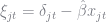
We can now consider the case when $\mu_{ijt} \neq 0$ . As with our naive model of demand, we are going to minimize a quadratic form in the unobserved product quality $\xi_{jt}$ . Our identifying assumption is that the expected unobserved quality is zero, conditional on observed product characteristics (excluding price). That is, $E[\xi_{jt} \vert x] = 0$ and so $E[Z(x)^{\prime}\xi \vert x] = 0$ , where $Z(x)$ is a set of instruments constructed from our data on product characteristics (as described above). With these moment conditions we can construct a GMM estimator for $\hat{\beta}$ , $\alpha$ , and $\sigma$ . The brute force way to solve this problem is to search over the parameter space and find the $(\hat{\beta}, \alpha, \sigma)$ that minimizes $(Z^{\prime}\xi)^{\prime}WZ^{\prime}\xi$ , where $W$ is an arbitrary weighting matrix. However, BLP’s method is more computationally efficient (this isn’t entirely true, see the literature on MPEC).

Berry (1994) demonstrated that $\delta$ is uniquely identified for a given set of parameter values $\alpha$ and $\sigma$ and a set of market share observations. Because $\delta$ is linear in $\hat{\beta}$ we can invert the system of equations to write $\hat{\beta}$ in terms of $\delta$ . Then $\xi_{jt} = \delta_{jt} - \hat{\beta} x_{jt}$ . This leads to the following algorithm:

Guess a set of parameter values for $\sigma$ and $\alpha$
Use a contraction mapping (see below) to solve for the $\delta$ that sets predicted shares equal to actual shares
Generate instrumental variable estimates of $\hat{\beta}$ given $\delta$ .
Use $\hat{\beta}$ to calculate $\xi$ and calculate the moment conditions

We then search over $\sigma$ and $\alpha$ and find the values that minimize the GMM objective function.

Simulation

In order to set the predicted market shares to the actual market shares we need to evaluate the following integral

$latex \displaystyle
s_j = \int \frac{\exp\{\delta_{j} + \mu_{ij}(\upsilon_i)\}}{\sum_l \exp\{\delta_{l} + \mu_{il}(\upsilon_i)\}} f(v_i)dv_i
$

where the $\upsilon_i$ are drawn from a mean zero normal distribution with identity covariance. This integral does not have a closed form solution and so we need to approximate it. BLP’s original paper proposes evaulating this through simulation. They use the simple smooth estimator (which is also referred to as a pseudo-Monte Carlo estimator in the literature)

$latex \displaystyle
\hat{s}_j = \frac{1}{n} \sum_{i = 1}^n \frac{\exp\{\delta_{j} + \mu_{ij}(\upsilon_i)\}}{\sum_l \exp\{\delta_{l} + \mu_{il}(\upsilon_i)\}}
$

This simulator works by analytically integrating out the extreme value errors and then evaluating the integrand at $ns$ draws from the standard normal distribution and averaging. This method appears to be the one most commonly used in empirical work. We can take draws from the standard normal with the following code. Note that income is assumed to be distributed lognormal, so we actually take $K + 1$ draws and use one of the draws to sample the income distribution. The lognormal distribution is assumed to have the following means (which change by year) and standard deviation (which is constant across years).

# Estimated means and deviations for lognormal distribution
incomeMeans = [2.01156, 2.06526, 2.07843, 2.05775, 2.02915, 2.05346, 2.06745,
2.09805, 2.10404, 2.07208, 2.06019, 2.06561, 2.07672, 2.10437, 2.12608, 2.16426,
2.18071, 2.18856, 2.21250, 2.18377]

sigma_v = 1.72

srand(719345)
ns = 1500
v_ik = randn(6,  ns )'
m_t = repeat(incomeMeans, inner = [ns, 1])

y_it = exp(m_t + sigma_v * repeat(v_ik[:,end], outer = [length(incomeMeans),1]));

unobs_weight = ones(ns)'/ns

Random Utility Term

Following Nevo (2001), I define a function called sim_mu which calculates the random terms in the utility function, $\mu_{ijt}$ . Recall that our utility function is given by

$latex \displaystyle
u_{ij} = \alpha \ln(y_i – p_j) + x_j \bar{\beta} + \xi_j + \sum_k \sigma_k x_{jk} \upsilon_{ik} + \epsilon_{ij}
$

The random term is therefore $\mu_{ijt} = \alpha \ln(y_i - p_j) + \sum_k \sigma_k x_{jk} \upsilon_{ik}$ . One issue that needs to be dealt with, which isn’t discussed in BLP (1995) but is mentioned in BLP (1999), is how to handle prices that are greater than a consumer’s income. The log of a negative number is not defined so we need an approximation. Note that

$latex \displaystyle
\alpha \ln( y_i – p_j) = \alpha \ln \left(y_i \left(1 – \frac{p_j}{y_i} \right) \right) = \alpha \ln (y_i) + \alpha \ln \left(1 – \frac{p_j}{y_i} \right)
$

The Taylor series expansion of the log function gives us

$latex \displaystyle
\ln( 1 + x ) = x – \frac{1}{2}x^2 + \frac{1}{3}x^3 + …
$

which we can substitute for the second term above,. Therefore, our approximation (after dropping higher order terms) to the original formula is given by

$latex \displaystyle
\alpha \ln( y_i – p_j) \approx \alpha \ln (y_i) – \alpha \frac{p_j}{y_i}
$

The left-hand side has support $\mathbb{R}_{++}$ while the right-hand side has support $\mathbb{R}$ .

In the below code we only include the term $- \alpha \frac{p_j}{y_i}$ and we include a random coefficient on the constant. This stems from the fact that we assume the outside good has utility

$latex \displaystyle
u_{i0t} = \alpha \ln (y_i) + \xi_{0t} + \sigma_0 \upsilon_{i0} + \epsilon_{0it}
$

We calculate choice probabilities by normalizing $u_{i0t}$ to be $0$ . This involves subtracting $\alpha \ln (y_i)$ from all of the inside good utilities. Note also that we need to subtract $\sigma_0 \upsilon_{i0}$ . We are implicitly doing this by giving the constant term a random coefficient. This part is not very clear in BLP’s original paper, although it is mentioned in footnote $6$ .

I use a Basic Linear Algebra Subroutine (BLAS) function to calculate the random terms. This was just to speed up the code and hopefully doesn’t add too much confusion. I calculate the random coefficients in two steps. First, I calculate new coefficients $(-\alpha / y_{it}, \sigma_1 \upsilon_1, ..., \sigma_k \upsilon_k)$ . Second, I multiply each coefficient by its respecitve product characteristic and sum together. BLAS.axpy!(a, x, y) is a function that replaces the value $y$ with $a\cdot x + y$ .

function sim_mu(x2, params)
    # Initialize Variables to be used in the calculation
    sub = Float64[]
    count = 0
    incomeDif = zeros(size(x2)[1], ns)
    mu = zeros(size(x2)[1], ns)
    coeffs = similar(params)
    params = abs(params)

    for m in marks
        tmp = find(markets .== m)
        count += 1 # Keep track of the number of markets
        sub = x2[find(markets .== m), :] # Product Characteristics for market m
        y = y_it[ns*(count-1)+1:ns*(count), :] # Get current income observations
        v = v_ik

        for i = 1:ns
            y_im = y[i]
            v_i = v[i,1:end-1]

            mu_ijt = zeros(size(sub)[1],1)
            # Part 1
            incomeDif[find(markets .== m), i] = y_im  # Needed for later calculations

            # Part 2
            coeffs[1] = - params[1] / (y_im)
            coeffs[2:end] = params[2:end] .* v_i
            for j in 1:size(sub)[2]
                BLAS.axpy!(coeffs[j] , sub[:,j], mu_ijt )
            end
            # Store the random effects part
            mu[tmp, i] = mu_ijt
        end
    end
    return [exp(mu), incomeDif]
end
@time test = sim_mu( [p convert(Array{Float64,2}, X)], [39.501,  3.612, 0.628, 1.818, 1.050, 2.056]);

Calculating Shares

The function calc_share is straightforward. For each consumer, in each market, it calculates the choice probabilities when given both a vector representing $\delta_{jt}$ and matrix representing $\mu_{ijt}$ . Note that both of these arguments need to be exponentiated. This is for efficiency reasons that I describe below.

function calc_share(expdelta, expmu)
    # Calculate the Market Shares
    # Combine the average effect with the individual random effect
    u_ijt = expdelta .* expmu
    p_ijt = zeros(size(u_ijt)...)

    for m in marks
        numer = view(u_ijt, find(markets .== m), : )

        prob = numer ./ (1+sum(numer, 1))
        p_ijt[find(markets .== m), :] = prob
    end

    # Calculating market shares
    s_jt = p_ijt * unobs_weight' #/ ns

    return [s_jt, p_ijt]
end
@time test2 = calc_share( exp(delta_0), test[1]);

The Contraction Mapping

The contraction mapping outlined in BLP is given by

$latex \displaystyle
\delta_{t+1} = \delta_{t} + \ln s_{act} – \ln s_{est}(\delta_t)
$

From a computational stand point, Nevo (2000) recommends using the transformation

$latex \displaystyle
e^{\delta_{t+1}} = e^{\delta_{t}} \frac{s_{act}}{s_{est}(\delta_t)}
$

It should be clear that if the former converges the latter will as well. Exponentials are less expensive to calculate than logarithms, and so this can speed up run times. Nevo reports that these are on the order of 10% although I haven’t bothered to test this assertion. It should be noted that much of the random coefficients literature is concerned with finding ways to avoid the contraction mapping. The most significant contribution that is asymptotically equivalent to BLP’s original model is Dube, Fox, and Su’s mathematical program with equilibrium constraints (MPEC). While MPEC uses the KNITRO solver (which you will need a license to use) it runs much faster than the “nested fixed point” method proposed by BLP.

function contraction( delta, x2, theta2w)
    mu = sim_mu( x2, theta2w )[1]

    delta0 = exp(delta)
    eps = 1
    act_share = convert(Array{Float64,1}, regSet[:share] ) ### Need to make more general
    count = 0
    flag = 0
    while (count  .0001 &amp;amp;amp;amp;amp;&amp;amp;amp;amp;amp; flag == 0)
        s_0 = calc_share(delta0, mu)[1]

        delta1 = delta0 .* (act_share ./ s_0)
        eps = maximum(abs((s_0./act_share) - 1))
        delta0 = delta1
        count += 1
        flag = sum(delta0 . 0
    end
    return log(delta0) 

end
@time newDelta2 = contraction( (delta_0), [p convert(Array{Float64,2},X)],  [39.501,  3.612, 0.628, 1.818, 1.050, 2.056] )

Calculating Marginal Costs

The above code is sufficient if you are only interested in modeling the demand side. However, estimates may be made more precise if a supply side is also incorporated. Recall from the initial problem set-up that profits for firm $f$ are given by

$latex \displaystyle
\Pi_f = \sum_{j \in \mathcal{F}_f} (p_j – mc_j) M s_j(p,x,\xi;\theta)
$

The first order conditions are given by

$latex \displaystyle
s_j(p,x,\xi;\theta) + \sum_{k \in \mathcal{F}_f} (p_j – mc_j) \frac{\partial s_j(p,x,\xi;\theta)}{\partial p_k} = 0
$

where the $M$ drops out as it is common to both terms in the above expression. Denoting the matrix of partial derivatives as $\Delta$ we can solve for the vector of marginal costs as

$latex \displaystyle
mc = p – \Delta^{-1} s(p,x,\xi;\theta)
$

The market shares formula is given by

$latex \displaystyle
s_{jt}(p, x, \xi, \theta, P_0) = \int p_{jt}(v_i, \delta(x, p, \xi), p, x, \theta) P_0(dv)
$

The own-price elasticity is given by the percent change in quantity to a percent change in price. We therefore need to differntiate the market shares with respect to price. Note that the differntiation operator passes through the integral, and so we just need to calculate the derivative of the choice probabilities and then integrate over these. Derivatives take a convenient form for logit models. Remember that the probability of choosing an option with observed characteristic $V_i$ is equal to

$latex \displaystyle
P_{ij} = \frac{e^{V_{ij}}}{\sum_k e^{V_{ik}}}
$

Taking derivatives with respect to some characteristic $x_{ij}$ gives

$latex \displaystyle
\frac{\partial P_{ij}}{\partial x_{ij}} = \frac{\partial V_{ij}}{\partial x_{ij}}\frac{e^{V_{ij}}}{\sum_k e^{V_{ik}}} – \frac{\partial V_{ij}}{\partial x_{ij}}\left(\frac{e^{V_{ij}}}{\sum_k e^{V_{ik}}}\right)^2
$

$latex \displaystyle
\frac{\partial P_{ij}}{\partial x_{ij}} = \frac{\partial V_{ij}}{\partial x_{ij}} P_{ij}(1-P_{ij})
$

Using this formula, we can see that the derivative of the market shares formula with respect to price is given by

$latex \displaystyle
\frac{\partial s_{jt}}{\partial p_{jt}} = \int \frac{\partial \mu_{ijt}}{\partial p_{jt}}p_{jt}(v_i, \delta(x, p, \xi), p, x, \theta)(1 – p_{jt}(v_i, \delta(x, p, \xi), p, x, \theta)) P_0(dv)
$

Remember that $p_{jt}$ only enters $\mu_{ijt}$ through $\alpha \ln (y_i - p_{jt})$ , so $\frac{\mu_{ijt}}{p_{jt}} = -\frac{\alpha}{y_i }$ .

It can be shown in an analogous manner that the cross-price derivative is given by

$latex \displaystyle
\frac{\partial s_{jt}}{\partial p_{qt}} = \int -\frac{\partial \mu_{iqt}}{\partial p_{qt}}p_{jt}(v_i, \delta(x, p, \xi), p, x, \theta) p_{qt}(v_i, \delta(x, p, \xi), p, x, \theta) P_0(dv)
$

Replacing the integral by sums and dividing by the number of simulated individuals (called $ns$ above) gives the estimated own and cross price derivatives.

function calc_mc(incomeDif, p_ijt, params)
    mc_all = zeros(delta_0)
    alpha = abs(params[1])
    s_jt = p_ijt * unobs_weight' #/ ns

    for m in marks
        firm_yr = firms[find(markets .== m),:]
        price = p[find(markets .== m)]
        income = incomeDif[find(markets .== m),:]
        sameFirm = convert(Array{Float64, 2}, firm_yr .== firm_yr')
        yr = p_ijt[find(markets .== m),:]

        nobs = size(yr)[1]
        grad = zeros(nobs, nobs)
        for i=1:ns
            grad .+= alpha ./ income[:,i] .* sameFirm .* unobs_weight[i] .* (yr[:,i].*yr[:,i]' - diagm(yr[:,i]))
        end
        subMatrix = - grad #/ ns
        b = inv(subMatrix) * s_jt[find(markets .== m),:]

        mc = price - b
        mc[mc.&amp;amp;amp;amp;lt;0] = .001
        mc_all[find(markets .== m), :] = mc
    end
    return mc_all
end
@time t4 = calc_mc(test[2], test2[2], 39.501)

The moment conditions for the GMM function need to be augmented. We do this by creating a block diagonal matrix of the instruments and a block diagonal matrix of the demand and supply structural errors and then interact these two terms together (see the function ObjFunc below).

Minimizing the GMM Objective Function

We can implement BLP’s algorithm with the four function above. It appears that BLP use a two step estimation technique. First, they use an identity weighting matrix and calculate initial consistent estimates. With these initial consistent estimates they redraw their random sample using importance sampling (which I will discuss later) and calculate the optimal GMM weighting matrix. They then rerun the algorithm to arrive at their final estimates using the new random draws and weighting matrix.

using NLopt

w1 = eye(size(z,2)) # You can change this to a different initial weighting matrix
preMult = inv(zxw'w1*zxw)*zxw'w1*z'
function gmm( y )
    bxw = preMult*y;
    return bxw
end

function ObjFunc(theta_2::Vector, grad::Vector)
        m.guess = contraction(m.guess, [m.price m.X], theta_2)
        mu, iD = sim_mu([m.price m.X], theta_2 )
        p_ijt = calc_share(exp(m.guess), mu )[2]
        mc = calc_mc(iD, p_ijt, theta_2[1])
        y = vcat(m.guess, log(mc))

        bxw = gmm( y )
        xi_w = y - xw*bxw
        g = z'xi_w/size(xi_w,1)
        quadForm = (g'w1*g*34)[1]
        println(theta_2, ", ", quadForm)
        return quadForm

end

opt = Opt(:LN_COBYLA, 6)
lower_bounds!(opt, [5.0, 0., 0., 0., 0., 0.])
initial_step!(opt, [3, .5, .5, .5, .5, .5].*.5)
xtol_rel!(opt,1e-2)
maxeval!(opt, 300)
min_objective!(opt, ObjFunc)

@time (minf,minx,ret) = NLopt.optimize(opt, [43.501,  3.612, 4.628, 1.818, 1.050, 2.056])

1007.059921 seconds (823.74 M allocations: 577.395 GB, 32.29% gc time)
(21.80850345845785,[25.3377,0.355161,4.18467,3.44204,0.820002,1.80589],:XTOL_REACHED)

Approximate Optimal Weighting Matrix

theta_2 = minx 

preMult = inv(zxw'w1*zxw)*zxw'w1*z'
function gmm( y )
    bxw = preMult*y;
    return bxw
end

m.guess = contraction(delta_0, [m.price m.X], theta_2)
mu, iD = sim_mu([m.price m.X], theta_2 )
p_ijt = calc_share(exp(m.guess), mu )[2]
mc = calc_mc(iD, p_ijt, theta_2[1])
y = vcat(m.guess, log(mc))

bxw = gmm( y )
xi_w = y - xw*bxw

g_ind = z.*xi_w

g = mean(g_ind,1)
vg = g_ind'g_ind/size(xi_w,1) - g .* g'

weight = inv(vg)

preMult = inv(zxw'weight*zxw)*zxw'weight*z'

Re-estimate Parameters

function ObjFunc(theta_2::Vector, grad::Vector)
        m.guess = contraction(m.guess, [m.price m.X], theta_2)
        mu, iD = sim_mu([m.price m.X], theta_2 )
        p_ijt = calc_share(exp(m.guess), mu )[2]
        mc = calc_mc(iD, p_ijt, theta_2[1])
        y = vcat(m.guess, log(mc))

        bxw = gmm( y )
        xi_w = y - xw*bxw
        g = z'xi_w/size(xi_w,1)*2
        quadForm = (g'weight*g*34)[1]
        println(theta_2, ", ", quadForm)
        return quadForm

end

opt = Opt(:LN_COBYLA, 6)
lower_bounds!(opt, [5.0, 0., 0., 0., 0., 0.])
initial_step!(opt, [3, .5, .5, .5, .5, .5] * .5)
xtol_rel!(opt,1e-1)
maxeval!(opt, 300)
min_objective!(opt, ObjFunc)

@time (minf2,minx2,ret2) = NLopt.optimize(opt,  [43.501,  3.612, 4.628, 1.818, 1.050, 2.056]  )

692.216123 seconds (522.84 M allocations: 437.516 GB, 35.45% gc time)
(14.393336822730385,[42.4779,2.51149,4.43821,4.17829,0.0253246,1.80782],:XTOL_REACHED)

These estimates are highly sensitive to the seed that you choose for your random number generator. The price coefficient is the only one that appears to be stable, as it is generally in the range of $38$ to $47$ . Adding more draws would help of course, however the program slows down significantly as more draws are added.

Computational Notes

Given the model set-up there is a significant discontinuity in the objective function when $\alpha$ becomes small enough. The easiest way to see this is to decompose the objective function into two parts, the portion due to the demand equations and the portion due to the supply equations. The magnitude of the demand moments are less sensitive to changes in $\alpha$ and the $\sigma_k$ s than the demand moments are, and as $\alpha$ gets small the supply moments dominate the objective function. That is until all marginal costs are set to $1$ (the lower bound that we put on the marginal costs). Because the dependent variable is constant, it can be approximated so well that the supply moments have a negligible contribution to the GMM function. At this point, changes in the $\sigma_k$ have an imperceptible impact on the supply moments and can be used to push down the demand moments. This leads to a global minimum of the GMM function with $\alpha \approx 1$ . This is of course economically unrealistic and more a facet of the lower bound we are forced to put on marginal costs. There are a few ways to avoid this result.

Use a smaller step size in the optimization routine. BLP uses the Nelder-Mead algorithm which uses an initial step size. If you make the step size sufficiently small, then it will converge to an economically relevant minimum. Of course, a smaller step size can lead to convergence to a local minimum and so you will need to start from a number of different points to make sure the algorithm is converging to the global minimum.
Use more draws or use a different form of numerical integration to approximate the tails better. Parameter values are largely determined by the tails of the distributions and better approximations of these tails leads to more rapid increases in the GMM objective function. The majority of the issues that I found came from using Monte Carlo methods with too few draws.

Numeric Integration

Judd and Skrainka (2011) propose using quadrature to estimate the integral instead. Quadrature evaulates the function at predetermined points called nodes and then calculates a weighted sum of the results, where the weights depend in a complex way on the nodes and the function you are integrating against. Fortunately there are Julia packages available that calculate quadrature nodes and weights for certain types of integrals. Because we are interested in integrating against a normal distribution we can use Gauss-Hermite quadrature for our approximation. The new estimator becomes

$latex \displaystyle
\hat{s}_j = \pi^{-\frac{K+1}{2}} \sum_{i = 1}^n \frac{\exp\{\delta_{j} + \mu_{ij}(\upsilon_i)\}}{\sum_l \exp\{\delta_{l} + \mu_{il}(\upsilon_i)\}} \cdot w_i
$

(you can see this result derived in the one-dimensional case here). One advantage of using quadrature instead of simulation is that we need fewer nodes to get similar levels of precision. Given that the number of draws is one of the biggest determinants of run time, the savings can be significant. One detriment is that the weights can be negative, leading to negative shares. This is problematic when computing the contraction mapping. The contraction mapping requires that the shares remain positive and sum to one, so if any share becomes negative it will diverge to $-\infty$ . This occurs more frequently as you increase the number of nodes you use, as the tails of the distribution become better approximated. Judd and Skrainka use MPEC to estimate the random coefficients model which avoids the contraction mapping and is therefore more robust to use with quadrature based rules.

I was a bit imprecise earlier when I said that the weights can be negative. Traditional quadrature actually has non-negative weights, but requires the integrand to be evaluated at a significant number of nodes. An alternative is to use sparse grid quadrature, which takes advantage of the normal distributions symmetry to calculate nodes and weights. The trade off is that you need to use fewer nodes but the weights may be negative. We can use calculate the nodes and weights using the Julia package SparseGrids. Again, note the normalization in calculating the nodes and weights.

using SparseGrids

Dim = size(X,2) + 1
nodes, weigths = sparsegrid(Dim,5,kpn)
ns = length(weigths)
v_ik = nodes' * sqrt(2)
unobs_weight = weigths' / sqrt(pi)^Dim

# Estimated means and deviations for lognormal distribution
sigma_v = 1.72

m_t = repeat(incomeMeans, inner = [ns, 1])

# Calculate Sample Incomes
y_it = exp(m_t + sigma_v * repeat(v_ik[:,end], outer = [length(incomeMeans), 1]));

To give a sense of how quadrature compares to pseudo-Monte Carlo methods I used a sparse grid approximation of order 5 (so it will integrate polynomials up to 9 degrees precisely). The first stage estimates were

447.178553 seconds (594.09 M allocations: 328.282 GB, 17.68% gc time)
(16.322633430097962,[35.9758,3.23863,5.49839,1.61946,0.843252,2.87426],:XTOL_REACHED)

and the second stage estimates were

222.237679 seconds (270.54 M allocations: 171.822 GB, 17.26% gc time)
(11.138638590017912,[43.5579,4.29131,6.5701,0.240026,0.878732,3.13293],:XTOL_REACHED)

The estimates are very similar to those generated from the pseudo-Monte Carlo draws (the coefficient on price is very close to what BLP estimates). The primary difference is the run time. Because we only need 749 points for the quadrature the estimation routine runs in roughly half the time. However, the reason that I used a rule of order 5 is not innocuous. As I tried to increase the order for more precision I began to frequently run into negative shares.

In his book “Discrete Choice Methods with Simulation” Kenneth Train suggests using Halton draws to evaluate this integral (this is an excellent book and provided online here). The random draws used for the pseudo-Monte Carlo estimator are serially uncorrelated. While this is not an issue for estimation it does mean that simulation errors tend to die out slowly. Halton draws are a way to create pseudo-random draws that are negatively correlated, which in effect cause the simulation errors to decrease more rapidly. You will often get similar levels of precision to the pseudo-Monte Carlo estimates with a tenth of the number of draws (see Bhat (2001)). The drawback is that the theoretical properties of using Halton draws have note been investigated and so it is an open question as to how they might impact your results, e.g. introducing bias or inconsistency, etc. For a discussion on using Halton Draws, see Train’s book in Chapter 9. The algorithm that I use below is based on the Wikipedia entry, found here.

using StatsFuns
#Pkg.add("Primes")
using Primes

function Halton(i = 1, b = 3)
    f = 1 # value
    r = 0
    while i &amp;amp;amp;amp;gt; 0
        f = f / b
        r = r + f * mod(i, b)
        i = floor(i/b)
    end
    return r
end

function HaltonDraws( k=6, n = 100, primeList = [3, 7, 13, 11, 2, 5])
    draws = zeros(n, k)
    myPrimes = primeList
    for j = 1:k
        draws[:,j] = [norminvcdf( Halton(i, myPrimes[j]) ) for i = 50:50+n - 1]';
    end
    println(myPrimes)
    return draws
end

ns = 2000
v_ik = HaltonDraws(6, ns)
unobs_weight = ones(1, size(v_ik, 1))/ns

# Estimated means and deviations for lognormal distribution
sigma_v = 1.72

m_t = repeat(incomeMeans, inner = [ns, 1])

# Calculate Sample Incomes
y_it = exp(m_t + sigma_v * repeat(v_ik[:,end], outer = [length(incomeMeans), 1]));

I ran the estimation routine using 1000 Halton draws using a random sequence of prime numbers (actually a random permutation of the first $6$ prime numbers). Here are the results

423.846489 seconds (374.58 M allocations: 244.325 GB, 37.97% gc time)
(24.47760690688335,[30.5585,2.00234,2.77162,3.27645,0.317881,0.0],:XTOL_REACHED)

and the second stage estimates were

310.120252 seconds (231.79 M allocations: 171.579 GB, 39.66% gc time)
(14.616969374249717,[43.4435,2.11105,3.44915,2.02088,0.299518,0.455816],:XTOL_REACHED)

Halton draws do appear to perform better than the pseudo-Monte Carlo draws. They also appear to compare favorably to quadrature and avoid the issue of negative market shares. However, there is till a large variation when it comes to choosing the order of your primes. Below is a selection of 20 different permutations using $2,000$ draws each.

[3,13,5,7,11,2]
(8.436375185058576,[39.7409,4.80046,3.02638,4.30049,0.043742,2.16608],:XTOL_REACHED)
[3,2,5,7,13,11]
(8.126970330811496,[38.379,4.98949,3.22361,5.87349,4.57709e-18,5.55112e-19],:XTOL_REACHED)
[11,2,13,3,7,5]
(8.281354450784724,[47.1244,4.25148,3.60036,1.89378,1.51985e-19,1.02716e-33],:XTOL_REACHED)
[5,7,13,3,11,2]
(8.004086471346755,[40.3787,5.07477,3.86652,4.73931,0.333077,1.59143],:XTOL_REACHED)
[3,7,13,5,2,11]
(8.806204934089184,[45.8064,3.46805,4.48342,2.39208,0.344699,2.06688],:XTOL_REACHED)
[5,13,2,3,11,7]
(7.91977691414021,[49.3665,3.60608,5.75227,2.88326,0.213072,1.63706],:XTOL_REACHED)
[11,5,2,3,13,7]
(8.199763136939843,[43.1127,4.3867,4.54713,4.2257,0.0609809,2.77556e-19],:XTOL_REACHED)
[13,7,3,5,11,2]
(8.141588621576702,[48.4785,4.59091,3.84852,2.00489,0.249055,0.302077],:XTOL_REACHED)
[3,5,11,13,2,7]
(8.037840784698098,[41.2783,4.62048,4.9107,4.7229,6.93889e-18,2.16878],:XTOL_REACHED)
[2,7,3,11,13,5]
(8.314772240236219,[49.3797,1.76477,1.23341,4.22146,6.93889e-18,2.63216],:XTOL_REACHED)
[11,2,13,3,7,5]
(8.389703007299477,[41.7569,4.55971,4.56189,2.0751,0.155372,1.15924],:XTOL_REACHED)
[5,11,13,2,3,7]
(7.311091187054691,[50.6297,3.23043,1.95696,6.12793,5.51136e-19,1.48309],:XTOL_REACHED)
[3,13,7,2,11,5]
(7.975776111976936,[51.1548,0.0,5.90186,4.70691,2.77556e-19,2.65734],:XTOL_REACHED)
[13,11,5,7,3,2]
(7.4030259001242085,[50.6504,4.69235,1.27391,4.75771,0.24332,0.842979],:XTOL_REACHED)
[3,13,11,5,2,7]
(8.141840785186503,[45.6043,4.95684,5.2669,2.32044,0.0,2.71834],:XTOL_REACHED)
[7,3,5,2,13,11]
(8.198262419497787,[44.0319,4.47802,1.85758,5.59819,0.0,0.525004],:XTOL_REACHED)
[2,13,3,5,7,11]
(8.094371918095108,[42.5261,3.64256,6.31567,5.40118,0.0456037,2.36173],:XTOL_REACHED)
[3,13,7,11,2,5]
(7.636265599411301,[45.3401,1.96728,7.69974,4.29029,5.20417e-20,3.74455],:XTOL_REACHED)
[13,5,7,3,11,2]
(7.296827100901245,[47.8753,4.23547,2.93748,3.77012,0.131486,3.23347],:XTOL_REACHED)
[3,5,7,11,13,2]
(8.143417852613503,[46.539,4.29459,6.11534,3.23859,0.0,1.32306],:XTOL_REACHED)

Standard Errors

BLP report that asymptotic standard errors take the form

$latex
(\Gamma^{\prime}\Gamma)^{-1}\Gamma^{\prime}\left(\sum_{i=1}^3 V_i\right)\Gamma(\Gamma^{\prime}\Gamma)^{-1}
$

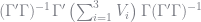
where

$latex
\Gamma = \frac{\partial \mathbb{E}[Z^{\prime}\xi(\theta)]}{\partial \theta}
$

See BLP (1995) for the definitions of the $V_i$ s. It is difficult to find an analytic solution for this derivative. We therefore use a numeric approximation. For each parameter we increase it by a small amount and then calculate the change in the objective function. We only do this for $\alpha$ and $\sigma$ as $\bar{\beta}$ has an analytic form that we can use. The term $V_1$ is just our standard GMM optimal weighting matrix. BLP ignore $V_2$ in their calculations and use Monte Carlo methods to estimate $V_3$ . I did not do this last part, although they report that it can increase standard errors by $5\%-20\%$ .

theta_2 = minx2
m.guess = contraction(m.guess, [m.price m.X], theta_2)
mu, iD = sim_mu([m.price m.X], theta_2 )
p_ijt = calc_share(exp(m.guess), mu )[2]
mc = calc_mc(iD, p_ijt, theta_2[1])
y = vcat(m.guess, log(mc))

bxw = gmm( y )
base_xi_w = y - xw*bxw

de = zeros( size(xw, 1), length(minx2) )
ident = eye( length(minx2) )

for i=1:length(minx2)
    theta_2 = minx2 + ident[:,i] * .01 * minx2[i]
    m.guess = contraction(m.guess, [m.price m.X], theta_2)
    mu, iD = sim_mu([m.price m.X], theta_2 )
    p_ijt = calc_share(exp(m.guess), mu )[2]
    mc = calc_mc(iD, p_ijt, theta_2[1])
    y = vcat(m.guess, log(mc))

    bxw = gmm( y )
    xi_w = y - xw*bxw

    de[:,i] = (xi_w - base_xi_w) / (.01 * minx2[i])
end

de2 = hcat(de, -xw)
Gamma = z'de2/(size(g_ind,1))
GammaInv = inv(Gamma'Gamma)

g_ind = z.*base_xi_w
g = mean(g_ind,1)
vg = g_ind'g_ind/(size(g_ind,1)) - g.*g'

variance= GammaInv *Gamma'*vg*Gamma*GammaInv / (size(g_ind,1))
standardErrors = sqrt(diag(variance))

hcat(vcat(minx2, bxw), standardErrors )

17×2 Array{Real,2}:
 42.4779      16.1789    
  2.51149      3.41254   
  4.43821      5.59275   
  4.17829      1.90392   
  0.0253246    0.58236   
  1.80782      1.92754   
 -7.08578      0.374612  
  2.74746      0.579396  
 -1.53175      0.10079   
  0.429704     0.0718583 
  3.60274      0.191931  
  1.96949      0.199927  
  0.470318     0.0686119 
  0.757718     0.0273383 
 -0.469276     0.130125  
 -0.365715     0.197932  
  0.00724009   0.00193253

One thought on “Random Coefficients (BLP)”

Alfred Fai SAM says:

March 10, 2019 at 10:59 am

That it great and helpful illustration on the computation details on BLP model! Thanks very much! However, I am so interested in how to use MPEC to solve for BLP model under Julia environment. If one more blog can introduce such topic, then we can compare the MPEC results with traditional results and see the benefits. Thanks very much again!

LikeLike