Random Coefficients and Importance Sampling

I’ve had a lot of difficulty getting robust estimates from my random coefficient models. It is frequently the case that merely changing the random number generator seed leads to large changes in my parameter estimates. This reflects the fact that simulation error is often a significant contributor to one’s standard errors. While generally unappealing in academic research, it is disastrous in a professional setting where point estimates tend to play an outsized role. The goal of this post is to introduce some methods to ameliorate the impact of simulation error and help make estimates more precise.

Berry, Levinsohn, and Pakes (1995) decompose the variance of their random coefficient estimator into three parts: variance from the product characteristics, variance from consumer sampling, and variance from simulating market shares. While we generally cannot eliminate the variance from the first two sources, the researcher has control over the last. With enough computing power, the simulation error could be driven to zero by taking an increasing number of random draws. Unfortunately, most researchers don’t have access to a supercomputer and must settle for using a small number of draws (I generally see people use between 50 and 5,000). The hope is that even with few draws the simulation error will be negligible. However, this is rarely the case. In their 1995 paper, BLP estimated that simulation error increased their standard error by around 5-20% and even doubled the standard error of one parameter. They were already using a variance reduction technique, so the situation would be worse using the industry standard pseudo-Monte Carlo techniques. Part of the problem is that Monte Carlo methods are inefficient. Adding an an additional decimal place of precision requires increasing the number of draws by a factor of 100. In problems where market shares are on the order of 0.001 (as in BLP) one would need to use millions of draws in order to get accurate estimates. Several techniques have been proposed in the literature to remedy this issue.

The simplest variance reduction method is to replace the Monte Carlo draws with a low discrepancy sequence, such as Halton sequences (e.g. Brunner (2017)), Sobol sequences (e.g. Li, et. al. (2017)), or Modified Latin Hypercube Sampling (e.g. Hess et. al. (2006)). These sequences provide a better coverage of the region of integration and can often achieve a variance similar to Monte Carlo integration with a fraction of the draws. In a the same vein, Skrainka and Judd (2011) proposed using sparse grid integration and monomial rules to approximate the market share integrals. While highly effective for lower dimensional problems, I have found this method does not work as well when there are many competitors. The reason is that with many competitors, market shares tend to be small and small market shares are determined by the tails of the distribution, exactly where the approximation is poorest. The focus of this page is importance sampling. This was the method used in Berry, Levinsohn, Pakes (1995), as well some of the subsequent random coefficients literature, e.g. Petrin (2002) and Petrin, Seo (2016)). More recently, Brunner (2017) proposed using a Gaussian importance sampler, another case I will consider below. When done properly, importance sampling can lead to significantly increases in efficiency for fewer draws. Unfortunately, it is also more difficult to implement reliably.

These notes rely heavily on my code for the random coefficient estimator, provided here. For a discussion of the mechanics of the BLP estimator (including using quadrature and Halton draws to approximate market shares), see the notes I posted here.

A Simple Example of Importance Sampling

Monte Carlo methods are straightforward, both to program and understand. What they lack in efficiency, they make up for in robustness. With enough time and computational power any integral can be accurately simulated and so any random coefficients model can be solved. Of course, efficiency is almost always a concern, necessitating the use of other methods. My previous post focused on using low discrepancy sequences and quadrature to reduce simulation error. BLP instead use importance sampling. Importance sampling, being as much art as science, lacks the same concreteness as Monte Carlo methods, requiring more care on behalf of the researcher to ensure that the resulting estimator is robust while simultaneously reducing computational complexity. Importance sampling has the potential to provide accurate results using few draws, however, when poorly implemented, it can make an estimator’s once finite variance, infinite.

To illustrate, consider taking $N$ draws from a standard normal distribution and estimating the probability that a given draw is greater than 4. The true probability of this occurring is approximately $0.00317\%$ , meaning we would expect about one observation above this threshold in $31,500$ draws. Using pseudo-Monte Carlo methods to estimate this probability accurately would require millions of draws. You can imagine a situation in which evaluating a function at a million different points would become prohibitive. Importance sampling ameliorates this problem by drawing from a more informative distribution and then weighting the draws to generate an integral numerically identical to the original. Let $h(y)$ be a function of the random variable $y$ , which has pdf $f(y)$ . We want to calculate the expected value of this function, but $f(y)$ might be difficult to draw from. Next assume that there is a candidate pdf $g(y)$ that shares the same support as $f(y)$ and is non-zero, then we can approximate $E[h(y)]$ as follows

$\displaystyle E[h(y)] = \int h(y)f(y) dy = \int \frac{h(y)f(y)}{g(y)}g(y)dy \approx \frac{1}{n}\sum \frac{h(y_i)f(y_i)}{g(y_i)}$

Note that the draws $y_i$ are taken from the pdf for $g$ . A good candidate transformation will have the same support as your original distribution but will take more draws from the region of interest. In our above example, we would like to take draws where $X > 4.0$ . As such, we let $g$ be the normal distribution with mean $4$ and standard deviation $1$ .

impSamp — **The blue distribution is our target distribution. The red is the candidate distribution.**

I calculated the frequency estimator using $1,000,000$ draws and the importance sampling estimator using $1,000$ draws, both $100$ times. The frequency estimator had a mean probability of $3.15e^{-5}$ and a standard deviation of $5.798816e^{-6}$ . The importance sampling estimator had a mean probability of $3.192491e^{-5}$ and a standard deviation of $2.07711e^{-6}$ . That is the strength of a well chosen importance sampling estimator: using fewer draws, the estimator is more accurate and has a lower variance. However, this example also highlights a potential pitfall. If we used a normal distribution centered around $-4$ , our estimator would not only be far less accurate, but it would also have a much higher variance than the pseudo-Monte Carlo estimator. So choosing a candidate distribution requires a lot of care.

The data generating process in BLP shares similarities with the above example. The market shares are small, with an average share of $0.00097$ , meaning that the market share integrals will need many Monte Carlo draws to approximate accurately. In BLP, the market shares are given by

$\displaystyle s_j = \int f_j(\nu)p(\nu)d\nu$

where $p(\nu)$ is multivariate normal with zero mean and a diagonal covariance matrix.

Importance Sampling in BLP

The Monte Carlo approach entails drawing $n$ draws from a standard normal distribution, and then using these draws to construct the random coefficients, $\beta_i = \beta + \nu_i \sigma$ . The Law of Large Numbers ensures that as $n$ goes to infinity, the average of these draws will approach the expected value, i.e. the expected market share. This is the standard method used in the vast majority of the literature.

$\displaystyle s_j = \frac{1}{n}\sum f_j(\nu_i)$

Consider the following transformation

$\displaystyle s_j = \int \frac{f_j(\nu)}{h(\nu)}p(\nu) h(\nu) d\nu$

where $h(\nu)$ has the same support as $f_j(\nu)$ and is itself a pdf. Then we can define the new function

$\displaystyle f_{hj} = \frac{f_j(\nu)}{h(\nu)}p(\nu)$

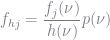
and note that integrating this function with respect to the pdf $h$ results in an identical expected value. If $h(\nu)$ could be found such that it was proportional to $f_j(\nu)p(\nu)$ , then $f_{hj}$ would be a constant, and so any simulator of the above integral would have zero variance! We would therefore have no simulation error and would be able to estimate the integral of interest exactly. Of course, we will almost never know the correct $h$ , so in practice this can only help us make an informed guess. If we knew the true value of $\theta_0$ , then we would choose an $h$ equal to

$\displaystyle h_j(\nu) = \frac{f_j(\nu)p(\nu)}{s_j(\nu; \theta_0)}$

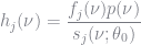
Here, we divide by $s_j(\theta_0)$ so that $h_j$ is a density. If we knew $\theta_0$ , we would be able to draw from this density using an accept-reject procedure. First, take draws from $p(\nu)$ (in this case the standard normal distribution) and construct $f_j(\nu_i)$ . Then take draws from the uniform distribution and accept $\nu_i$ if $u_i < f_j(\nu_i)$ . The resulting draws represent the conditional distribution of $\nu$ , given that $U < f_j(\nu)$ . We can establish that this distribution is the distribution of $h_j(\nu)$ .

Let $H_j(\nu)$ be the cdf of $h_j$ and define the following sets, conditional on $\nu$ .

$\displaystyle A = \left\{U < f_j(Y)\right\}\\ B = \left\{Y < \nu\right\}\\$

Note that

$\displaystyle P(A) = P\left(U \leq f_j(Y) \right) = \int_{-\infty}^{\infty}P\left(U \leq f_j(Y) \vert Y = \nu \right)p(\nu)d\nu$

The term inside the integral is equal to $f_j(\nu)$ (because we are conditioning on $\nu$ , so this integral simplifies to

$\displaystyle \int_{-\infty}^{\infty}P\left(U \leq f_j(Y) \vert Y = \nu \right)p(\nu)d\nu = s_j(\theta)$

Next, we need to calculate $P(B)$ , but that is just equal to $\Phi(\nu)$ . Finally, we need to calculate $P(A \vert B)$ , which is simply

$\displaystyle P(A\vert B) = \frac{P\left(U \leq f_j(Y), Y \leq \nu \right)}{\Phi(\nu)}$

Conditioning and integrating, and noting that $P(U \leq f_j(Y)\vert Y) = f_j(Y)$ by the properties of the uniform distribution, gives

$\displaystyle \frac{P\left(U \leq f_j(Y), Y \leq \nu \right)}{\Phi(\nu)} = \frac{1}{\Phi(\nu)}\int_B f_j(\nu)p(\nu)d\nu$

With these probabilities in hand, we can apply Bayes Rule.

$\displaystyle P(B\vert A) = \frac{P(B)}{P(A)} P(A \vert B) = \frac{\Phi(\nu)}{s_j(\theta)\Phi(\nu)} \int_B f_j(\nu)p(\nu)d\nu = \int_B \frac{f_j(\nu)}{s_j(\theta)}p(\nu)d\nu$

By the last term is equal to $H_j(\nu)$ . So this accept-reject procedure lets us draw from $H_j(\nu)$ .

We don’t know $\theta_0$ , but we can use an initial consistent estimate of it, $\hat{\theta}$ , and then draw from that density instead. If $\hat{\theta}$ is close to $\theta_0$ , then $h_j$ will be close to its optimal value, and our importance sampler will be very efficient. This is similar to optimal GMM. We first use a consistent, but inefficient, estimate of $\theta$ to calculate the optimal weighting matrix, and then re-estimate $\theta$ with this matrix to get a more efficient estimator.

There is one last thing to note. The optimal $h_j$ depends on $j$ , i.e. there is an optimal $h$ for each market share we are approximating. We typically don’t use a different importance sampler in practice, so we choose one that works well for all market shares. BLP use the probability of purchasing a car, i.e. $1 - s_0$ . In the above discussion, we just need to replace $f_j(\nu)$ with $\sum_{j \in J} f_j(\nu)$ and $s_j(\theta)$ with $1 - s_0(\theta)$ . The draws are then the same for all models within the market.

The theory is involved, but coding the importance sampler is actually quite simple. The first thing we need is an initial consistent estimate. I use the parameter values reported in BLP. Given our consistent estimate $\theta$ , we need to calculate $\delta(\theta)$

βs = [-7.061, 2.883, 1.521, -0.122, 3.46]
γs = [0.952, 0.477, 0.619, -0.415, -0.046, 0.019]
α = 43.501
σs = [3.612, 4.628, 1.818, 1.050, 2.056];

srand(1234)

ns = 5000*20
v_ik1 = randn(6,  ns )'

# Antithetic draws, for shits and giggles
v_ik1 = reshape([v_ik1[:] -v_ik1[:]]', size(v_ik1,1)*2, size(v_ik1,2))
m_t = repeat(incomeMeans, inner = [ns*2, 1])
 
y_it1 = exp.(incomeMeans .+ sigma_v * v_ik1[:,end]');

unobs_weight = ones(ns*2)'/(ns*2)*20;

The first step, the call to gen_mm2, calculates the $\delta$ from our initial consistent estimate. This is the $\delta$ which will determine the mean utility of all the products for the purposes of importance sampling. Then, for each market, we calculate the average $\bar{s} = 1 - s_0$ using a large number of draws (determined by the parameter nsi). As noted in BLP, we only need to calculate $\bar{s}$ once, which means we can use a large number of draws to accurately approximate the integral. Next, we take nf draws from the uniform distribution and the standard normal distribution. We calculate $\bar{f}(\nu_i) = \sum_j f_j(\nu_i)$ for each draw and determine if $u_i \leq \bar{f}(\nu_i)$ . If this condition holds, we accept the draws and create the sampling weight $w_i = \frac{\bar{f}(\nu_i)}{\bar{s}}$ . Otherwise we reject the draw and continue. This process repeats until we have exactly nf draws per market.

function impSample(m::ModelData, nsi::Int64, nf::Int64)

    m_t = [2.01156, 2.06526, 2.07843, 2.05775, 2.02915, 2.05346, 2.06745,
            2.09805, 2.10404, 2.07208, 2.06019, 2.06561, 2.07672, 2.10437, 2.12608, 2.16426,
            2.18071, 2.18856, 2.21250, 2.18377]
    sigma_v = 1.72
    ns = nf * length(m_t)
    xdraws = zeros(ns, size(m.X,2))
    ydraws = zeros(ns)
    weight = zeros(ns)
 
    # Calculate Share
    for ms in unique(m.marketidx)
        clock = 0
        idx1 = m.midx[ms,1]; idx2 = m.midx[ms,2]
        X = m.X[idx1:idx2,:]
        p = m.price[idx1:idx2]
        draws = randn(size(X,2)+1, nsi)
    
        randci = X * (draws[1:end-1,:] .* m.sigma)
        y_it = exp.(m_t[ms] + sigma_v * draws[end,:])'
        
        uijt = randci .- p./y_it * m.alpha .+ m.delta[idx1:idx2]
        renorm = maximum(uijt, 1)
        uijt .= exp.(uijt .- renorm)
        share = uijt./(exp.(-renorm)+sum(uijt,1))
        s_avg = mean(sum(share,1))

        count = 1
        while (nf >= count )*(10000 > clock)
            clock += 1
            tdraws = randn(size(X,2)+1, nf)
            randci = X * (tdraws[1:end-1,:] .* m.sigma)
            y_it = exp.(m_t[ms] + sigma_v * tdraws[end,:])'

            uijt = randci .- p./y_it * m.alpha .+ m.delta[idx1:idx2]
            renorm = maximum(uijt, 1)
            uijt .= exp.(uijt .- renorm)
            share = uijt./(exp.(-renorm)+sum(uijt,1))
            
            share = sum(share,1)
            udraws = rand(nf)

            for i = 1:nf
                if udraws[i]  nf
                    break
                end
            end
        end
    end
    weight = weight / ns * size(m.midx,1)
    return xdraws, ydraws, weight
end

The importance draws should result in a lower variance in estimating market shares. The BLP estimator sets market shares to their observed values, so we are more interested in the variance of the implied $\delta$ . I compared the mean standard deviation of $\delta$ , for 20 different sets of draws, for Monte Carlo integration and BLP’s importance sampler. I used the following code for the importance sampling.

N = 20
dtest2 = zeros(length(m.delta), N)
for i = 1:N
    m = ModelData(  price[:], X, α, βs, γs, σs, deepcopy(delta_0), deepcopy(delta_0), markets[:], midx, J_f, y_it, v_ik[:,1:end-1], 
      unobs_weight'[:], zeros(size(X,1), size(v_ik,1)/20), convert(Array{Float64,1}, deepcopy(d_share)), 
        convert(Array{Float64,1}, deepcopy(d_share)), deepcopy(delta_0), zeros(size(X,1), 19));
    m.y_it = 1.0./m.y_it[m.marketidx,:];
    srand(i)
    v_ik1, y_it1, unobs_weight1 = impSample(m, 8000, 750);
    # Correct the y_it draws
    incy = 1.0./exp.(incomeMeans .+ sigma_v * y_it1')[m.marketidx,:];
    m2 = ModelData(  price[:], X, α, βs, γs, σs, deepcopy(delta_0), deepcopy(delta_0), markets[:], midx, J_f, incy, v_ik1, 
          unobs_weight1, zeros(size(X,1), size(v_ik1,1)/20), convert(Array{Float64,1}, deepcopy(d_share)), 
            convert(Array{Float64,1}, deepcopy(d_share)), deepcopy(delta_0), zeros(size(X,1), 19));
    gen_mm2(m2)
    dtest2[:,i] = deepcopy(m2.delta)
end

mean((std(dtest2,2)))

0.2238364471487058

The standard Monte Carlo method, with the same number of draws, gave a mean standard deviation of 0.731. So we reduce the standard deviation of $\delta_j$ by a factor of 3. On its face, this seems pretty good. However, in my experience, this is rarely a large improvement on low discrepancy sequences and barely lowers the standard deviation of the actual parameter estimates. Your mileage may vary. My preferred method currently is adaptive importance sampling, which I will turn to next. It is more computationally intensive, for the same number of draws, but consistently leads to much lower standard errors.

Gaussian Importance Sampling

The BLP importance sampler requires taking draws from a non-normal distribution using an accept-reject method that is not guaranteed to generate a sample in a reasonable amount of time. So that’s not great. An alternative approach, proposed by Brunner (2017) and based on the work of Heiss (2010), would be to find the normal distribution that best approximates $f_j(\nu)\phi(\nu)$ and use it for our $h$ . They call this technique adaptive efficient importance sampling, or adaptive EIS. More explicitly, consider re-weighting the market share integral as

$\displaystyle s_j = \int \frac{f_j(\nu_{r}; \theta)\phi(\nu_{r})}{\phi(L^{-1}(\nu_{r} - a))}\phi(L^{-1}(\nu_{r} - a))d\nu = \int \frac{f_j(a + Lx; \theta_0)\phi(a + Lx)}{\phi(x)}\phi(x) \vert L \vert dx$

where the term $\vert L \vert$ comes from the change in variable. We can approximate this integral using standard pseudo-Monte Carlo draws. We take draws from the standard normal distribution, evaluate $f_j$ at $Lx + a$ and then weight these values by $\vert L \vert \frac{\phi(a + Lx)}{\phi(x)}$ . The question is, can we find values of $L$ and $a$ that minimize the variance of the above approximation. Unfortunately we can’t; not without knowing the value of $\theta_0$ . However, as with BLP’s importance sampler, we can use a consistent estimate of $\theta_0$ to approximate the optimal $L$ and $a$ . Define the following distance

$\displaystyle e = \ln \left(\frac{f(\nu_r)\phi(\nu_r)}{\phi(L^{-1}(\nu_{r} - a))} \right) + c$

where $c$ is an irrelevant constant. Using the definition of the standard normal distribution, this distance is equal to

$\displaystyle e_r = \ln f(\nu_r) - \frac{1}{2}\nu_r^{\prime}\nu_r + \frac{1}{2}(\nu_r - a)^{\prime}B^{-1}(\nu_r - a) - c$

where $B^{-1} = \left(LL^{\prime}\right)^{-1}$ . We can expand this error term to get a linear system of equations

$\displaystyle \ln f(\nu_r) - \frac{1}{2}\nu_r^{\prime}\nu_r = c - \frac{1}{2}a^{\prime}B^{-1}a^{\prime} - \frac{1}{2}\sum_i b_{ii}\nu_{ri}^2 - \frac{1}{2}\sum_{i\neq j} b_{ij}\nu_{ri}\nu_{rj} + \nu_r^{\prime}B^{-1}a + e_r$

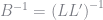
Defining

$\displaystyle \alpha = c - \frac{1}{2}a^{\prime}B^{-1}a^{\prime}\\ \beta_{ii} = 2 b_{ii}\\ \beta_{ij} = b_{ij}\\ \gamma = B^{-1}a$

we can run a weighted regression of $\ln f(\nu_r) - \frac{1}{2}\nu_r^{\prime}\nu_r$ on a constant and the levels and second order interactions of the components of $\nu_{r}$ to find the values of $\alpha$ , $\beta$ , and $\gamma$ that minimize the following weighted squared distance

$\displaystyle \min_{a,L}\ \sum_r e_r^2 f_j(\nu_r) w_r$

Using the estimates for $\beta$ we can recover $B^{-1}$ and then $L$ , by taking the Cholesky factorization of its inverse. With estimates of $B^{-1}$ and $\gamma$ we can calculate $a$ as well. We therefore have all the information we need for our importance sampler.

With estimates of $L$ and $a$ in hand, we calculate our new expectation using standard techniques. Importantly, we can use additional variance reduction techniques to approximate the new integral. Brunner (2017) uses Halton draws and Heiss (2010) uses sparse grid quadrature. Here, I use Modified Latin Hypercube Sampling draws as they are quick and easy to calculate, and perform well with the automobile data.

There is one last subtlety that needs to be discussed before implementation. In both the BLP and adaptive EIS methods we need an initial estimate of $\delta$ to calculate market shares. In BLP, they use the initial consistent estimate of $\theta$ and a large number of draws to get an estimate of $\delta(\theta)$ that has little simulation error. This $\delta$ provides the mean utility for importance sampling. However, because $\theta$ , and therefore $\delta(\theta)$ , change at each step in our GMM procedure, our draws will not be optimal apart from the initial consistent estimate. We can’t redraw the optimal importance sample at each step however, because then our GMM objective function function will be infinitely jumpy and we will never get convergence. Adaptive EIS, on the other hand, works by adapting the same set of draws. That is, for a fixed set of draws $\{\nu_{ik}\}$ , we can recalculate the optimal $L$ and $a$ for any given $\theta$ . This means that we could technically repeatedly update $L$ and $a$ in the contraction mapping, using the new value of $\delta$ at each step. Because calculating $L$ and $a$ is computationally expensive, this is not an optimal strategy, but we can still approximate it by calculating them for the first $n$ steps of the contraction. Brunner proposed updating them for the first 5 iterations, which I have found works well with the BLP data. Another strategy would be to set a tolerance, say 0.01, so that when the contraction error is small you stop updating the coefficients. This would ensure that the $\delta$ you use to adapt your draws is close to the true value. The strategies are virtually indistinguishable in practice.

function gen_mm3(m::ModelData, seed::Int64)
    α = m.alpha
    v_ik = m.v_ik
    J_f = m.J_f
    midx = m.midx
    for i = 1:length(m.p_ijt)
        m.p_ijt[i] = 0.0
    end
  
        # precalculate income effect
    m.delta .= exp.(m.delta)
        
    step = Int(size(m.v_ik,1)/20)
    n = step
    srand(seed)
    ns = n * length(unique(m.marketidx))
    xdraws = zeros(ns, size(m.X,2)); ydraws = zeros(ns); weight = zeros(ns)
    
    n_ = size(m.X,2)+1
    d = MvNormal(zeros(n_), eye(n_))

    m_t = [2.01156, 2.06526, 2.07843, 2.05775, 2.02915, 2.05346, 2.06745, 2.09805, 2.10404, 2.07208, 2.06019, 2.06561, 2.07672, 2.10437, 2.12608, 2.16426, 2.18071, 2.18856, 2.21250, 2.18377]
    sigma_v = 1.72
    
    X_ = Array{Float64,2}(0,0)
    lng = Array{Float64,2}(0,0)
    t1 = collect(0:n - 1) / n;
    
    # iterate over markets
    for mi = 1:size(m.midx,1)
        r1 = midx[mi,1]; r2 = midx[mi,2];
        muidx1 = step*(mi - 1) + 1; muidx2 = step*mi
        hs = rand(n_)/n

        totd = zeros(n,n_)
        for j = 1:n_
            th = t1 + hs[j]
            th = th[randperm(n)]
            totd[:,j] = [norminvcdf( th[i] ) for i = 1:n]';
        end
        
        draws = totd'
        
        d2 = sum(draws .* draws,1)/2.0;
        v_ik = draws[1:end-1, :]'
        y_it = exp.(m_t[mi] + sigma_v * draws[end,:])'
        
        X = m.X[r1:r2,:]

        δhat = m.delta[r1:r2]
        pt = m.price[r1:r2]
        mui = X*(v_ik.*m.sigma')' .- m.alpha*pt./y_it
        mui = exp.(mui)
  
        eps = 1.0; count = 1
        
        numer = zeros(mui)

        # contraction mapping/fixed point
        while (eps > 1e-14)*(200 > count)

            if 6 > count
                myin = δhat'mui
                pijt = myin ./ (1.0 + myin)
                lng = log.(pijt)
        
                y_ = (lng .- d2)[:]

                is0 = find(y_ .!= -Inf)

                X_1 = zeros(n , Int(n_*(n_+1)/2))
                idx = 1
                for i = 1:n_
                    for j = i:n_
                        X_1[:,idx] .= draws'[:,i].*draws'[:,j]
                        idx += 1
                    end
                end
                X_ = hcat(ones(n), draws', X_1)
                X_ = X_[is0,:]
                y_ = y_[is0]
                gw = pijt[is0]' 

                Δs = ((X_.*gw)'X_)\(X_.*gw)'y_

                γs_ = Δs[2:n_+1]
                tmp = zeros(n_,n_)
                idx = 1
                for i = 1:n_
                    for j = i:n_
                        tmp[i,j] = Δs[n_+2:end][idx]
                        if i == j
                            tmp[i,j].*=2
                        end
                        idx+=1
                    end
                end

                B = inv(Symmetric( -tmp ))

                L = chol(Hermitian(B))';

                a = B*γs_;

                vs = draws

                somed = L*vs .+ a

                m.v_ik[muidx1:muidx2,:] .= somed[1:end-1,:]'
                m.y_it[mi, muidx1:muidx2] .= 1./exp.(m_t[mi] + sigma_v*somed[end,:])
                m.unobs_weight[muidx1:muidx2] .= pdf(d, somed) ./ pdf(d, vs) * det(L) / n#.* unobs_weight
                mui2 = X*(m.v_ik[muidx1:muidx2,:] .*m.sigma')' .- m.alpha*pt.*m.y_it[mi, muidx1:muidx2]'
                mui2 = exp.(mui2)
            end

            numer .= mui2.*δhat;
            s0 = 1.0./(1.0 + sum(numer,1))
            m.p_ijt[r1:r2,:] .= numer .* s0;

            m.s_jt[r1:r2] .= m.p_ijt[r1:r2,:] * m.unobs_weight[muidx1:muidx2]
            
           # Finding the Fixed Point
            if eps > 0.1
                # Nevo Contraction
                m.delta[r1:r2] .= m.delta[r1:r2] .* m.act_s[r1:r2]./m.s_jt[r1:r2]
   
                eps = maximum(abs.((m.s_jt[r1:r2]./m.act_s[r1:r2]) - 1))
    
            else
                # Newton Root-finding
                m.delta[r1:r2] .= log.(m.delta[r1:r2])
                tmp2 = m.p_ijt[r1:r2,:] .* m.unobs_weight[muidx1:muidx2]'

                Jf = Base.LinAlg.I - (tmp2*m.p_ijt[r1:r2,:]')./m.s_jt[r1:r2,:]
                diff = log.(m.s_jt[r1:r2]) .- log.(m.act_s[r1:r2])
                stp = -Jf\diff
                m.delta[r1:r2] .= m.delta[r1:r2] .+ stp
                eps = maximum(abs.(stp))
                m.delta[r1:r2] .= exp.(m.delta[r1:r2])
            end
            δhat = m.delta[r1:r2]
            count += 1
        end

    end
    m.delta .= log.(m.delta)

    # calculate mc
    for j = 1:size(J_f, 1)
        
        idx1 = J_f[j,1]; idx2 = J_f[j,2];
        muidx = searchsortedlast(m.midx[:,1], idx1 )
        muidx_1 = (muidx-1)*step + 1
        muidx_2 = (muidx)*step
        rp = m.p_ijt[idx1:idx2,:] 
        wα =  m.unobs_weight[muidx_1:muidx_2] .* m.y_it[muidx,muidx_1:muidx_2] * α
        nfirms = idx2 - idx1 + 1;
        tmp2 = rp .* wα'
        tmpvec = diagm(rp * wα);
        gemm!('N', 'T', -1.0, m.p_ijt[idx1:idx2,:], tmp2 , 1.0, tmpvec) 

        b = tmpvec\m.s_jt[idx1:idx2]
        m.mc[idx1:idx2] .= m.price[idx1:idx2] .- b
    end
    for i = 1:length(m.mc)
        m.mc[i] = ifelse(0 > m.mc[i], 0.001, m.mc[i])
    end
    return nothing
end

Using the above code, I performed the same test as before and calculated the mean standard deviation of the $\delta$ s. Using the same number of draws, my mean standard deviation was

0.17706002102174695

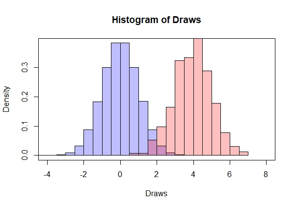
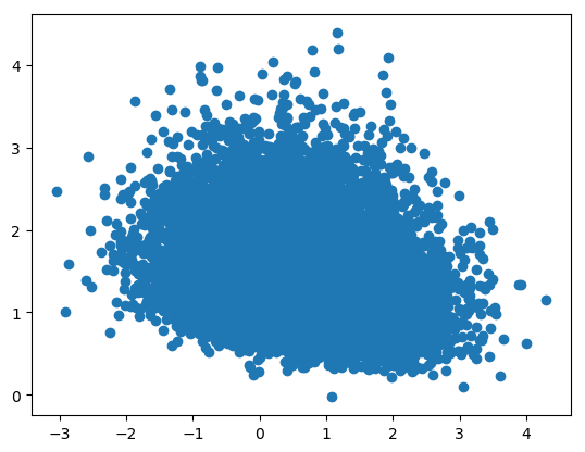
So adaptive EIS performed better than the baseline Monte Carlo and BLP’s importance sampler. To get a sense of how the two importance samplers work, I plotted a subset of the optimal draws for each method. The BLP draws are essentially bounded from below, reflecting the fact that it excludes draws that lead to a zero probability of purchasing one of the products. Adaptive EIS results in similar coverage, but includes those zero probability draws. In this sense, adaptive EIS is less efficient. However, by allowing the parameters $L$ and $a$ to vary based on the current value of $\delta(\theta)$ it actually results in superior coverage, and therefore a lower variance of $\delta$ .

EIS — **Adaptive Efficient Importance Sampling Draws**

Performance

I have shown that each method resulted in a lower variance for estimated $\delta$ when compared to standard Monte Carlo techniques. A more important question is how they impact the variance of parameter estimates. For each method, I estimated the first stage thirty times using 750 draws for simulation. For both importance samplers, I started with a “best case scenario”, using BLP’s reported estimates as my starting estimates.

std(tmpxMC2, 1) = [12.2137 2.34301 3.71322 1.38401 0.377048 1.54341]
mean(tmpxMC2, 1) = [42.0602 4.59074 4.01737 1.83184 0.421121 2.49259]
1×6 Array{Float64,2}:
 0.290385  0.510377  0.924291  0.755526  0.895344  0.619197

The results I got for the BLP importance sampler are not a significant improvement. The relative standard deviation do decrease uniformly for each parameter, however, the mean price coefficient is much larger than the BLP estimate. This is because the price coefficient is sensitive to outliers and BLP’s importance sampler is more likely to result in outliers. As the number of draws is increased, this problem goes away.

std(tmpx, 1) = [11.2117 2.3445 3.49407 0.988789 0.319127 1.41423]
mean(tmpx, 1) = [56.7875 4.13899 4.16129 1.86884 0.392125 2.62202]
1×6 Array{Float64,2}:
 0.197432  0.566444  0.83966  0.529093  0.813839  0.539366

The situation is improved with adaptive EIS. First note that the mean price parameter estimate is much closer to what BLP reported. Second, note that the relative standard deviation has decreased for most parameters and is substantially lower for the price coefficient $\alpha$ .

std(tmpx, 1) = [4.8542 1.14702 1.74645 1.05404 0.248643 0.724849]
mean(tmpx, 1) = [44.853 4.92704 4.07281 2.15881 0.293268 2.54106]
1×6 Array{Float64,2}:
 0.108225  0.2328  0.428806  0.48825  0.847836  0.285254

As with all estimation routines, there is a trade-off between speed and accuracy. Adaptive EIS is very accurate but takes considerably longer to estimate. This is because the optimal draws are updated multiple times in each step, as opposed to once at the beginning. For many problems, such as random coefficient models without income effects, the BLP importance sampler will work well and be much faster. As always, it is up to the researcher to try each and see what works best in the context of their question.

References

Berry, Steven, James Levinsohn, and Ariel Pakes. “Automobile prices in market equilibrium.” Econometrica: Journal of the Econometric Society (1995): 841-890.
Brunner, Daniel, “Numerical Integration in Random Coefficient Models of Demand” PhD diss., Universität Düsseldorf, 2017
Heiss, Florian. “The panel probit model: Adaptive integration on sparse grids.” Maximum simulated likelihood methods and applications. Emerald Group Publishing Limited, 2010. 41-64.
Hess, Stephane, Kenneth E. Train, and John W. Polak. “On the use of a modified latin hypercube sampling (MLHS) method in the estimation of a mixed logit model for vehicle choice.” Transportation Research Part B: Methodological 40.2 (2006): 147-163.
Li, Yang. An empirical study of national vs. local pricing under multimarket competition. Columbia University, 2012.
Petrin, Amil. “Quantifying the benefits of new products: The case of the minivan.” Journal of political Economy 110.4 (2002): 705-729.
Petrin, A., and B. Seo. “Identification and estimation of discrete choice models when observed and unobserved product characteristics are correlated.” (2016).
Skrainka, Benjamin S., and Kenneth L. Judd. “High performance quadrature rules: How numerical integration affects a popular model of product differentiation.” (2011).

A Simple Example of Importance Sampling

Importance Sampling in BLP

Gaussian Importance Sampling

Performance

References

Share this:

Like this:

Leave a Reply Cancel reply