Heterogeneous Agents with Aggregate Risk – Krusell/Smith

Note: To solve the heterogeneous agents model without aggregate risk, see my post on the Aiyagari model here.

Aiyagari type models can induce agents to save more than models with complete markets, however the level of savings is still much smaller than what we see in the data. While you can increase the savings rate by assuming larger values of risk aversion or income variability, there is little justification for these higher values. As Aiyagari writes,

“The quantitative results of this paper suggest that the contribution of uninsured idiosyncratic risk to aggregate saving is quite modest, at least for moderate and empirically plausible values of risk aversion, variability, and persistence in earnings.”

One possible explanation for the counterfactually low savings rate is that the standard Aiyagari model has no aggregate risk. The level of aggregate capital is known each period, resulting in a constant interest rate and wage. This implies that the only uncertainty that a consumer will face is with respect to their income process. It could be that adding in aggregate risk will make agents save even more, pushing up the aggregate savings rate and allowing us to better match the data.

Aiyagari excluded aggregate risk because it makes the problem far less tractable. Agents would need to not only forecast their individual state but also the distribution of assets in the economy (as that is what will determine prices in the subsequent period). But solving for a law of motion that moves any initial distribution forward one period and that is consistent with the optimal policy function is a daunting task. In their 1998 paper, “Income and Wealth Heterogeneity in the Macroeconomy,” Krusell and Smith (KS from now on) proposed a way to work around this problem and include aggregate risk. Rather than try and parameterize a transition function for the entire distribution, they assume that agents are boundedly rational and instead forecast moments of the distribution instead. Specifically, in their original paper, agents forecast the average level of capital $m_K$ using

$\ln m_{K,t+1} = \beta_0 + \beta_1 \ln m_{K,t}$

and assume that prices are determined by

$r = \alpha z_{s^{\prime}}\left(\frac{h_{\text{fix}}(1-u_{s^{\prime}})}{m_K} \right)^{1-\alpha} - \delta$

where $h_{\text{fix}}(1-u_{s^{\prime}})$ is the measure of aggregate labor (discussed further below). Now agents only need to know the current mean of the distribution to predict the mean next period, and the aggregate law of motion for capital reduces to a linear equation. While this makes the model feasible to solve, it is still a computationally difficult problem, as you will see in the code below.

Model Set-up and Parameterization

As is traditional in economic papers, we will be changing our baseline model slightly but will be changing the notation completely. For instance, Aiyagari writes $a_t$ for assets while KS use $k_t$ instead. I mention this because I used my Aiyagari code as a starting point for the KS algorithm and so my naming conventions are inconsistent across functions. I’m sorry if this confuses you, it confused me as well. The agent solves the following problem

$\max\ E_0 \left\{ \sum_t \beta^t U(c_t)\right\}\\ \\ \text{ s.t }c_t + k_{t+1} = w \epsilon h_{\text{fix}} + (1-\epsilon) b + (1+r) k_t$

where utility is given by

$U(c_t) = \frac{c_t^{1-\sigma} - 1}{1-\sigma}$

Here, $\epsilon$ is an indicator variable that determines if the agent is employed or not. This is the agent’s idiosyncratic shock. If they are employed they receive the wage times the number of hours they work (given by $h_{\text{fix}}$ ). If the agent is unemployed, they get some unemployment benefit $b$ .

The parameters that KS used to calibrate their model are given below. Note that $\beta$ is larger than what we used in the Aiyagari model, $\delta$ is smaller, and $\sigma$ is much smaller. Only $\alpha$ remains consistent.


β = 0.99

δ = 0.025

α = 0.36

σ = 1.00000

hfix = 0.3271 # Hours worked

homeY = 0.07 # The unemployment benefit

Aggregate prices are determined by a Cobb-Douglas production function

$r = \alpha z_{s^{\prime}}\left(\frac{h_{\text{fix}}(1-u_{s^{\prime}})}{m_k} \right)^{1-\alpha} - \delta$

where $1-u_s$ is the measure of employed workers, making $u_s$ the unemployment rate. The aggregate state is given by $z_s$ , which takes on one of two values: $z_h$ and $z_l$ . An important piece of the KS calibration is specifying the transition matrix for the idiosyncratic and aggregate states. There are two individual states (employed and unemployed) and two aggregate states (low and high), making a total of four potential states. The transition matrix is assumed to be Markov and the idiosyncratic and aggregate states are assumed to be correlated.

KS choose the probabilities to imply an unemployment rate of 4% in high states and 10% in low states. Let $u_s$ represents the unemployment rate in the current state. This means that the measure of agents that are currently employed is $1 - u_s$ and $u_s$ are unemployed. If $\pi_{ss^{\prime}00}$ is the probability of an unemployed individual being again unemployed next period (given the aggregate state moves from $s$ to $s^{\prime}$ ) and $\pi_{ss^{\prime}10}$ is the probability that a currently employed individual becomes unemployed, then the unemployment rate must satisfy

$u_s \frac{\pi_{ss^{\prime}00}}{\pi_{ss^{\prime}}} + (1-u_s) \frac{\pi_{ss^{\prime}10}}{\pi_{ss^{\prime}}} = u_{s^{\prime}}$

That is, the measure of unemployed agent’s next period is the probability of an unemployed agent being unemployed, times the measure of unemployed agents, plus the probability of an employed worker becoming unemployed, times the measure of employed workers. An equivalent formula must hold for the measure of employed workers. These have to hold for any aggregate state transition (e.g. low to low or high to low).

Of course, these restrictions alone are not sufficient to pin down the transition matrix. KS therefore impose a few additional restrictions. First, the average duration of an unemployment spell is $1.5$ quarters in good aggregate states and $2.5$ in bad aggregate states. If each period is a quarter, this implies that for good states

$\frac{1}{1-\pi_{gg00}} = 1.5$

and for bad states

$\frac{1}{1-\pi_{bb00}} = 2.5$

To see this, note that the probability of not getting a job in $t$ periods is equal to $\pi_{ss00}^t$ , for a given state $s$ . Therefore, the average duration is equal to

$E[\text{dur}] = \sum_{t=0}^{\infty} t \pi_{gg00}^t = \frac{1}{1-\pi_{gg00}}$

KS further impose

$\frac{\pi_{gb00}}{\pi_{gb}} = 1.25 \frac{\pi_{bb00}}{\pi_{bb}}$

and

$\frac{\pi_{bg00}}{\pi_{bg}} = 0.75 \frac{\pi_{gg00}}{\pi_{gg}}$

for reasons. The following code is largely lifted from the KS backup, although I changed some of the notation so that it is more consistent with their original paper.


urate = [0.1, 0.04, 0.1, 0.04]

durug = 1.5

unempg = 0.04

durgd = 8.0

durbd = 8.0

durub=2.5

unempb=0.1

πgg00 = (durug-1.0)/durug

πbb00 = (durub - 1.0)/durub

πbg00 = 1.25 * πbb00

πgb00 = 0.75 * πgg00

πgg01 = (unempg - unempg*πgg00)/(1.0-unempg)

πbb01 = (unempb - unempb*πbb00)/(1.0-unempb)

πbg01 = (unempb - unempg*πbg00)/(1.0-unempg)

πgb01 = (unempg - unempb*πgb00)/(1.0-unempb)

πgg = (durgd-1.0)/durgd

πgb = 1.0 - (durbd-1.0)/durbd

πgg10 = 1.0 - (durug-1.0)/durug

πbb10 = 1.0 - (durub-1.0)/durub

πbg10 = 1.0 - 1.25*πbb00

πgb10 = 1.0 - 0.75*πgg00

πgg11 = 1.0 - (unempg - unempg*πgg00)/(1.0-unempg)

πbb11 = 1.0 - (unempb - unempb*πbb00)/(1.0-unempb)

πbg11 = 1.0 - (unempb - unempg*πbg00)/(1.0-unempg)

πgb11 = 1.0 - (unempg - unempb*πgb00)/(1.0-unempb)

πbg = 1.0 - (durgd-1.0)/durgd

πbb = (durbd-1.0)/durbd

P0 =[

    πbb*πbb00 πgb*πgb00 πbb*πbb10 πgb*πgb10;

    πbg*πbg00 πgg*πgg00 πbg*πbg10 πgg*πgg10;

    πbb*πbb01 πgb*πgb01 πbb*πbb11 πgb*πgb11;

    πbg*πbg01 πgg*πgg01 πbg*πbg11 πgg*πgg11

]

4×4 Array{Float64,2}:
 0.525       0.03125     0.35      0.09375 
 0.09375     0.291667    0.03125   0.583333
 0.0388889   0.00208333  0.836111  0.122917
 0.00911458  0.0243056   0.115885  0.850694

As with any macro model, we need to define a grid over out state variables. The following code determines the grids over aggregate capital and cash-in-hand. KS observe that the policy functions are very flat in the aggregate capital dimension, so I use 6 grid point between 10 and 13. This choice comes from the benefit of foresight. Typically it is necessary to start with a wider grid, see where the aggregate capital tends to fall and then successively narrow the grid until you have a good approximation. The reported regression coefficients have implied steady-state values of aggregate capital for the low and high states of $11.34$ and $12.18$ , respectively. I therefore choose an interval that encompasses these values, is not too wide, but allows plenty of movement around the steady-state values.

I choose the grid over cash-in-hand analogously to my Aiyagari code. The lowest value is set to the cash-in-hand an unemployed worker with zero assets would have (KS assume that the agent gets a flow value of $0.07$ from home production). The maximum value is set at the maximum sustainable level of capital in the good aggregate state. In these models, a good initial guess for the savings policy function is some constant share of maximum allowed savings. Conveniently, the maximum amount an agent can save at any point on the cash-in-hand grid is the total cash-in-hand. This makes a good initial guess trivial for any of the potential states.


# Matrix of state values. First column is the aggregate state,

# second column is the individual state

fullY =[0.99 0.0;

        1.01 0.0;

        0.99 1.0;

        1.01 1.0];

# Grid over the aggregate state

āmin = 10.0

# Next to no curvature here, arbitrary maximum state size

āmax = 13.0

abargrid = collect(linspace(āmin, āmax, 6))

# Minimum potential wealth. KS assume agent's can earn 0.07 when unemployed

zmin = 0.07

# Max sustainable investment

kmax = (δ/fullY[2,1])^(1/((α-1)))

zmax = 1.01*kmax^α + (1-δ)*kmax

# Create grid over cash on hand. Add more points towards the origin

kgrid = collect(linspace(zmin^(1/30), zmax^(1/30), 50).^30)

# Maximum assets = cash-in-hand

maxa = zeros(length(kgrid), length(abargrid), 4)

for s = 1:4

    as = kgrid *(abargrid'./abargrid')

    maxa[:,:,s] = as - 0.001

end

Interpolation Object and Associated Functions

The interpolating object is more complicated than in the Aiyagari model, as we now need to keep track of both the aggregate state and a law of motion for this state. This requires adding a grid over aggregate capital and a grid for the distribution of assets. We also need to add regression coefficients which represent the agent’s best guess at the law of motion for aggregate capital. The below custom type stores all of the relevant variables.


# Interpolating Object

type GalerkinObj

    β::Float64

    δ::Float64

    α::Float64

    σ::Float64

    ζ::Float64

    ϕ::Float64

    hfix::Float64 # Average Hours

    homeY::Float64 # Home Production

    urate::Array{Float64,1} # Unemployment rates in good and bad states

    P::Array{Float64, 2} # Transition Matrix

    reg::Array{Float64, 2} # Regression Coefficients

    states::Array{Float64,2} # Potential States after shocks (both idiosyncratic and aggregate)

    θs::Array{Float64, 3} # FEM coefficients

    gridk::Array{Float64, 1} # Individual capital grid points

    gridK::Array{Float64, 1} # Aggregate Capital grid points

    agrid::Array{Float64, 1} # Distribution grid

    Kdist::Array{Float64, 1} # Distribution of Capital

    function GalerkinObj(β, δ, α, σ, ζ, ϕ, hfix, homeY, urate, P, reg, states, gridk, gridK, agrid)

        return new(β, δ, α, σ, ζ, ϕ, hfix, homeY, urate, P, reg, states, zeros(length(gridk), length(gridK), length(states)),

            gridk, gridK, agrid, zeros(length(agrid)*2))

    end

end

# Grid for distribution

agrid = collect(linspace(0.0, zmax, 300)); 

# My custom type

go = GalerkinObj(β, δ, α, σ, 0.0, 0.0, hfix, 0.07, urate, P0, [0.085 0.095; 0.965 0.962], fullY, kgrid, abargrid, agrid);

go.θs = maxa*0.98;

Interpolation is carried out using bilinear interpolation. Each grid point has an associated coefficient in our interpolating object. Any sample point will fall in the middle of four grid points. The below function takes two coordinates, x and y, and does a simple sorted search over the grids for individual capital and aggregate capital and returns the index of the grid point immediately before the sample coordinate. Using the indices of these lower grid points and their immediate successors we can determine the four coefficients that contribute to our interpolated value. Wikipedia has a good discussion on bilinear interpolation and provides various methods for calculating an interpolated value (see here).


function(itp::GalerkinObj)(x::Float64, y::Float64, s::Int64)

    gridx = itp.gridk

    gridy = itp.gridK

    indxl = min(max(searchsortedlast(gridx,x), 1), length(gridx)-1)

    indyl = min(max(searchsortedlast(gridy,y), 1), length(gridy)-1)

    yh = gridy[indyl+1];

    yl = gridy[indyl];

    xl = gridx[indxl];

    xh = gridx[indxl + 1]; 

    denom = (xh-xl)*(yh-yl)

    a11 = itp.θs[indxl, indyl, s]

    a12 = itp.θs[indxl, indyl+1, s]

    a21 = itp.θs[indxl+1, indyl, s]

    a22 = itp.θs[indxl+1, indyl+1, s]

    return (a11*(xh - x)*(yh - y) + a21*(x - xl)*(yh - y) + a12 * (xh - x)*(y - yl) + a22*(x-xl)*(y-yl))/denom

end

We will need to take the derivative of this interpolation object with respect to both the interpolation coefficients and the various arguments. These are easy to calculate, and I wrap them in the following two functions.


# Derivative for specific coefficient

function(itp::GalerkinObj)(d1::Int64, d2::Int64, x::Float64, y::Float64, s::Int64)

    gridx = itp.gridk

    gridy = itp.gridK

    indxl = min(max(searchsortedlast(gridx,x), 1), length(gridx)-1)

    indyl = min(max(searchsortedlast(gridy,y), 1), length(gridy)-1)

    yh = gridy[indyl+1];

    yl = gridy[indyl];

    xl = gridx[indxl];

    xh = gridx[indxl + 1]; 

    denom = (xh-xl)*(yh-yl)

    if (d1 == indxl)&(d2 == indyl)

        deriv = (xh - x)*(yh - y) / denom

    elseif (d1 == indxl+1)&(d2 == indyl)

        deriv = (x - xl)*(yh - y) / denom

    elseif (d1 == indxl)&(d2 == indyl + 1)

        deriv = (xh - x)*(y - yl) / denom

    elseif (d1 == indxl+1)&(d2 == indyl+1)

        deriv = (x-xl)*(y-yl) / denom

    else

        deriv = 0.0

    end

    return deriv

end


# Derivative for specific state

function(itp::GalerkinObj)(x::Float64, y::Float64, s::Int64, d::Int64)

    gridx = itp.gridk

    gridy = itp.gridK

    indxl = min(max(searchsortedlast(gridx,x), 1), length(gridx)-1)

    indyl = min(max(searchsortedlast(gridy,y), 1), length(gridy)-1)

    yh = gridy[indyl+1];

    yl = gridy[indyl];

    xl = gridx[indxl];

    xh = gridx[indxl + 1]; 

    denom = (xh-xl)*(yh-yl)

    a11 = itp.θs[indxl, indyl, s]

    a12 = itp.θs[indxl, indyl+1, s]

    a21 = itp.θs[indxl+1, indyl, s]

    a22 = itp.θs[indxl+1, indyl+1, s]

    if d == 1

        deriv = (-a11*(yh - y) + a21*(yh - y) - a12*(y - yl) + a22*(y-yl))/denom

    else

        deriv = (-a11*(xh - x) - a21*(x - xl) + a12 * (xh - x) + a22*(x-xl))/denom

    end

    return deriv

end

The Euler Equation and its Derivative

The Euler Equation does not change much between our original Aiyagari model and the KS model. The primary difference is that $r$ and $w$ are now state dependent and must therefore be brought inside the expectation for next period.

$R(z, s, \alpha) = (z - \hat{a}^{\prime})^{-\mu} - \zeta \min\{\hat{a}^{\prime},0\}^2 - \beta \sum_{s^{\prime}}\pi_{s, s^{\prime}}(1+r_{s^{\prime}}) (z^{\prime} - \hat{a}^{\prime\prime})^{-\mu}$

We again choose the coefficient in our finite element method to solve

$\int R(z, K, s, \alpha)\phi(z, K)_{s, i} dz = 0,\ \forall i = 1,...,N_k N_K$

where $\phi(z, K)_{s, i} = \phi(z)_{s,i}\phi(K)_{s,i}$ are our basis functions. Note that the multidimensional basis function is made up by taking the product of the unidimensional basis functions (for further discussion on the finite element method see Ellen McGrattan’s 1993 paper cited below and my Aiyagari code). Given a current aggregate capital and regression coefficients, the agent will predict tomorrows aggregate to be

$K^{\prime} = e^{\beta_{s,0} + \beta_{s,1} \ln K}$

Prices in the period will therefore be predicted to be

$r^{\prime} = \alpha z_{s^{\prime}}\left(\frac{h_{\text{fix}}(1-u_{s^{\prime}})}{K^{\prime} } \right)^{1-\alpha} - \delta$

$w^{\prime} = (1-\alpha) z_{s^{\prime}} \left(\frac{h_{\text{fix}}(1-u_{s^{\prime}})}{K^{\prime} } \right)^{-\alpha}$

Using this wage and interest rate we can calculate the implied cash-in-hand next period and use our current guess at the savings policy function to calculate implied consumption and savings.


function R_all(z::Float64, abar::Float64, s::Int64, â::GalerkinObj)

    ζ, σ, β, ϕ, δ, hfix, homeY, α, P, reg, urate =  â.ζ, â.σ, â.β, â.ϕ, â.δ, â.hfix, â.homeY, â.α, â.P, â.reg, â.urate

    ys = â.states

    â′ = â(z, abar, s)

    abar′ = exp(reg[1, mod(s+1, 2) + 1] + reg[2, mod(s+1, 2) + 1]*log(abar))

    lhs = 0.0

    rhs = (z - â′ )^(-σ) - ζ * min(â′, ϕ)^2

    for s′ = 1:size(ys, 1)

        r = α * ys[s′, 1] * (hfix*(1.0 - urate[s′])/abar′)^(1.0-α) - δ

        w = (1-α) * ys[s′, 1] * (abar′/(hfix*(1.0 - urate[s′])))^(α)

        z′s = w*ys[s′,2]*hfix + homeY*(1.0 - ys[s′,2]) + (1.0 + r)*â′ - r*ϕ

        â′′ = â(z′s, abar′, s′ )

        lhs += (1.0 + r)*(z′s - â′′)^(-σ)*P[s, s′]

    end

    lhs = β * lhs

    return rhs - lhs

end

The derivative with respect to a given coefficient is straightforward to calculate as well. Each coefficient can be associated with an index $i, j, z$ , where $i$ identifies it position in the individual assets grid, $j$ in the aggregate capital grid, and $z$ indexes the current state. We use the derivative function above to determine how our policy function changes with each coefficient. In order to determine how the entire residual changes, we need to take a total derivative again. The math is a bit messy, but gives the following result


function R′_all(dz::Int64, dabar::Int64, ds::Int64, z::Float64, abar::Float64, s::Int64, â::GalerkinObj)

    ζ, σ, β, ϕ, δ, hfix, homeY, α, P, reg, urate =  â.ζ, â.σ, â.β, â.ϕ, â.δ, â.hfix, â.homeY, â.α, â.P, â.reg, â.urate

    â_d = â(dz, dabar, z, abar, ds)

    ys = â.states

    â′ = â(z, abar, s)

    abar′ = exp(reg[1, mod(s+1, 2) + 1] + reg[2, mod(s+1, 2) + 1]*log(abar))

    rhs = σ*(z - â′ )^(-σ-1.0)*â_d*(ds==s) - ζ * 2.0 * min(â′, ϕ)*â_d*(ds==s)

    lhs = 0.0

    if ds == s

        for s′ = 1:size(ys, 1)

            r = α * ys[s′, 1] * (hfix*(1.0 - urate[s′])/abar′)^(1.0-α) - δ

            w = (1-α) * ys[s′, 1] * (abar′/(hfix*(1.0 - urate[s′])))^(α)

            z′s = w*ys[s′,2]*hfix + homeY*(1.0 - ys[s′,2]) + (1 + r)*â′ - r*ϕ

            â′′ = â(z′s, abar′, s′ )

            lhs += -(1+r)*σ*(z′s - â′′)^(-σ-1.0)*((1.0+r)*(â_d - â(z′s, abar′, s′, 1)*â_d) - â(dz, dabar, z′s, abar′, s′)*(s==s′)) * P[s, s′]

        end

    else

        r = α * ys[ds, 1] * (hfix*(1.0 - urate[ds])/abar′)^(1-α) - δ

        w = (1-α) * ys[ds, 1] * (abar′/(hfix*(1.0 - urate[ds])))^(α)

        z′s = w*ys[ds,2]*hfix + homeY*(1.0 - ys[ds,2]) + (1 + r)*â′ - r*ϕ

        lhs = -(1.0+r)σ*(z′s - â(z′s, abar′, ds))^(-σ-1.0)*( - â(dz, dabar, z′s, abar′, ds) ) * P[s, ds]

    end

    lhs = β*lhs

    return  rhs - lhs

end

One benefit of the Galerkin Method is that it leads to sparse Jacobians. This greatly reduces the computational cost of our Newton’s method, as we only need to calculate the values of a few specific elements in the matrix. Because we use bilinear interpolation, only four coefficients contribute to our interpolated value for any given point $(k_t, K_t)$ . In the below image, any point in the shaded block will have a value built up from the coefficients at the block’s corners. Therefore, the derivative of our policy function with respect to any most coefficients will be zero. In the example below, the blue point will have a non-zero derivative with respect to the four surrounding coefficients, and a zero derivative with respect to all other coefficients.

Bilinear Interpolation

Notice that the residual equation evaluates the policy function at $5$ points (one for the current state, and four for the potential future states). This all implies that our residual equation will have at most $20$ coefficients with non-zero derivative at a given point: four for the state in the current period, and four a piece for the four potential future states. For each weighted residual equation, we use two quadrature points in each dimension, making a total of $4$ . Therefore, for any one weighted residual equation, it will have at most $80$ non-zero entries, further implying that the Jacobian has at most $96,000$ non-zero entries in our example ( $50$ grid points for individual capital, times $4$ points for aggregate capital, times $4$ states, times $80$ ), or about 6.66% of the matrix elements are non-zero. However, this is actually somewhat of an overestimate. In my simple calculation, only about 2.95% of the elements were non-zero because a lot of $80$ coefficients per equation were redundant. Given a state, an expectation for the law of motion of capital, and a policy function we can therefore identify which coefficients will have a non-zero derivative for each weighted residual equation. The below function does exactly that, storing the indices in a matrix called tmp.

Quick computational note: For efficient code, the three steps that I just laid out – solving for the residual value, identifying non-zero elements in the Jacobian, and solving for the derivative – should all be combined in a single step. Note that many of the calculations that I have done (such as calculating the interest rate, or evaluating the policy function) are redundant. I break these steps out into individual functions for clarity, but ultimately this will not scale as well as a single piece of code where these steps are all combined.


function idcell2!(tmp::Array{Int64, 2}, z::Float64, abar::Float64, s::Int64, â::GalerkinObj)

    ζ, σ, β, ϕ, δ, hfix, homeY, α, P, reg, urate =  â.ζ, â.σ, â.β, â.ϕ, â.δ, â.hfix, â.homeY, â.α, â.P, â.reg, â.urate

    ys = â.states

    kgrid = â.gridk

    Kgrid = â.gridK

    count = 1

    # grid on capital

    idxz1 = min(max(searchsortedlast(kgrid, z), 1), length(kgrid)-1)

    idxbar1 = min(max(searchsortedlast(Kgrid, abar), 1), length(Kgrid)-1)

    abar′ = exp(reg[1, mod(s+1, 2) + 1] + reg[2, mod(s+1, 2) + 1]*log(abar))

    idxbar2 = min(max(searchsortedlast(Kgrid, abar′), 1), length(Kgrid)-1)

    # projected assets and state

    â′ = â(z, abar, s)

    for idz = idxz1:idxz1+1

        for idbar = idxbar1:idxbar1+1

            tmp[count, 1] = idz; tmp[count, 2] = idbar; tmp[count, 3] = s

            count += 1

        end

    end

    for idxbar = idxbar2:idxbar2+1

        for s′ = 1:size(ys, 1)

            r = α * ys[s′, 1] * (hfix*(1.0 - urate[s′])/abar′)^(1-α) - δ

            w = (1-α) * ys[s′, 1] * (abar′/(hfix*(1.0 - urate[s′])))^(α)

            z′s = w*ys[s′,2]*hfix + homeY*(1.0 - ys[s′,2]) + (1.0 + r)*â′ - r*ϕ

            idxz2 = min(max(searchsortedlast(kgrid, z′s), 1), length(kgrid)-1)

            for idxz′ = idxz2:idxz2+1

                if  (s′ == s)&(idxz′ == idxz1)&(idxbar == idxbar1)|

                    (s′ == s)&(idxz′ == idxz1+1)&(idxbar == idxbar1)|

                    (s′ == s)&(idxz′ == idxz1)&(idxbar == idxbar1+1)|

                    (s′ == s)&(idxz′ == idxz1+1)&(idxbar == idxbar1+1)

                    continue

                else

                    tmp[count, 1] = idxz′; tmp[count, 2] = idxbar; tmp[count, 3] = s′

                    count += 1

                end

            end

        end

    end

    return nothing

end

Weighted Residual and Newton’s Method

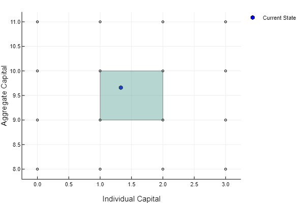
More care needs to be taken in two dimensions when constructing our weighted residual equation. Again, our weights are given by hat functions. Each hat function spans four individual elements (each different shade of green is an element in the image below). The hat function takes the value $1$ at the central grid point and $0$ at the boundaries. Therefore, each element will contribute to only four of the weighted residual equations. Rather than transversing the weighted residual equations and calculating their value one at a time, we will instead transverse the elements and calculate their contribution to the four relevant weighted residual equations. The reason we do this is because it avoids calculating our residual equation and its associate derivative at the same point multiple times.

Elements

The total number of elements is equal to the product of our grid dimensions, so by iterating over all grid points we will transverse all of the elements. The below code iterates over the states, the aggregate capital grid, and the individual capital grid and creates four indices at each step


idx1 = (s-1)*nk*nK + nk*(j-1) + i

idx2 = (s-1)*nk*nK + nk*(j-1) + i + 1

idx3 = (s-1)*nk*nK + nk*(j) + i

idx4 = (s-1)*nk*nK + nk*(j) + i + 1

These are linear indices that uniquely identify the four weighted residual equations that the current element contributes to. The function calculates the residual and its derivative at the four quadrature nodes, gives the values the appropriate weights, and then adds these values to the array position determined by the above indices. In this way, we build up the weighted residual values in a piece-wise fashion. I include four additional weights below, m1 – m4, which only serve to add more weight to the equations on the boundary. For instance, the weighted residual equations at the corners only have a single element contributing to their value, so I scale the calculated value by 4. All weighted residual equations will therefore have roughly 4 elements contributing to their value. I have found that this improved the stability of my Newton’s method.


function weightedResidual(go::GalerkinObj, N::Int64)

    nodes, weights = gausslegendre(N)

    resc1 = zeros(length(nodes))

    resc2 = zeros(length(nodes))

    w1 = zeros(length(nodes))

    w2 = zeros(length(nodes))

    Gθ = zeros(length(go.θs), length(go.θs))

    res = zeros(length(go.θs))

    tmp = zeros(Int64, size(go.states,1)*5, 3) # for check id of cells

    nk = length(go.gridk)

    nK = length(go.gridK)

    foridx = size(go.θs)

    eps = vec(go.θs); count = 0

    while (maximum(abs(eps)) > 1e-10)*(40 > count)

        count += 1

        # Reset Values to zero

        for i = 1:length(res)

            res[i] = 0.0

            for j = 1:length(res)

                Gθ[i,j] = 0.0

            end

        end

        # Iterate over states

        for s = 1:size(go.states,1)

             # iterate over grid points

            for j = 1:nK-1

               for i = 1:nk-1

                    kl = go.gridk[i] ; kh = go.gridk[i + 1];

                    Kl = go.gridK[j]; Kh = go.gridK[j+1];

                    denom = (kh - kl)*(Kh - Kl) # Denominator

                    for n = 1:length(nodes)

                        resc1[n] = (nodes[n]+1.0)*(kh-kl)/2.0 + kl

                        resc2[n] = (nodes[n]+1.0)*(Kh-Kl)/2.0 + Kl

                        w1[n] = weights[n]*(kh-kl)/2.0

                        w2[n] = weights[n]*(Kh-Kl)/2.0/denom

                    end

                    m1 = ifelse(i == 1, 2.0, 1.0)

                    m2 = ifelse(j == 1, 2.0, 1.0)

                    m3 = ifelse(i + 1 == nk, 2.0, 1.0)

                    m4 = ifelse(j + 1 == nK, 2.0, 1.0)

                    idx1 = (s-1)*nk*nK + nk*(j-1) + i

                    idx2 = (s-1)*nk*nK + nk*(j-1) + i + 1

                    idx3 = (s-1)*nk*nK + nk*(j) + i

                    idx4 = (s-1)*nk*nK + nk*(j) + i + 1

                    # Function

                   for k_ = 1:length(resc1)

                            for K_ = 1:length(resc2)

                                for tt = 1:length(tmp)

                                    tmp[tt] = 0

                                end

                                val = R_all(resc1[k_], resc2[K_], s, go)

                                weigh = w1[k_]*w2[K_]

                                res[idx1] += weigh*val*(kh - resc1[k_])*(Kh - resc2[K_])*m1*m2

                                res[idx2] += weigh*val*(resc1[k_] - kl)*(Kh - resc2[K_])*m2*m3

                                res[idx3] += weigh*val*(kh - resc1[k_])*(resc2[K_]-Kl)*m1*m4

                                res[idx4] += weigh*val*(resc1[k_] - kl)*(resc2[K_] - Kl)*m3*m4

                                idcell2!(tmp, resc1[k_], resc2[K_], s, go)

                                # Derivative

                                for c = 1:size(tmp,1)

                                    if tmp[c,1] != 0

                                        gs = tmp[c,3]; gj = tmp[c,2]; gi = tmp[c,1]

                                        idxd = (gs-1)*nk*nK + nk*(gj-1) + gi

                                        val = R′_all(gi, gj, gs, resc1[k_], resc2[K_], s, go)

                                        Gθ[idx1, idxd] += weigh*val*(kh - resc1[k_])*(Kh - resc2[K_])*m1*m2

                                        Gθ[idx2, idxd] += weigh*val*(resc1[k_] - kl)*(Kh - resc2[K_])*m2*m3

                                        Gθ[idx3, idxd] += weigh*val*(kh - resc1[k_])*(resc2[K_]-Kl)*m1*m4

                                        Gθ[idx4, idxd] += weigh*val*(resc1[k_] - kl)*(resc2[K_] - Kl)*m3*m4

                                    end

                                end

                            end

                        end

                    end    

            end

        end

        eps = -Gθ\res

        for i = 1:length(go.θs)

            go.θs[i] += eps[i]#*ifelse(count<5,0.5,1.0)

        end

    end

    for i = 1:length(go.θs)

        go.θs[i] = max(go.θs[i], 0.0)#*ifelse(count<5,0.5,1.0)

    end

    @show maximum(abs(eps))

    return nothing

end

go = GalerkinObj(β, δ, α, σ, 0.0, 0.0, hfix, 0.07, urate, P0, [0.085 0.095; 0.965 0.962], fullY, kgrid, abargrid, agrid);

go.ζ = 1000000.0

go.θs = maxa*0.98;

@time weightedResidual(go, 2)

Policy Function

Calculating the Distribution of Assets

I again use Young’s histogram method to determine the distribution of assets. KS use simulation, which is slower and less accurate. A problem that KS faced was that simulation could not force the unemployment rate to be $0.04$ in good states and $0.1$ in bad states. To remedy this, they had to pick random agents and switch their status from employed to unemployed (or vice versa) to achieve the target unemployment rate. Young’s method avoids this completely, as the unemployment rate is factored into the transition matrix and will therefore always be exact. Care needs to be taken when determining how fine the grid over individual capital is in the histogram method. Bin sizes less than $0.1$ are typically needed to have good convergence properties in our “contraction”. However, having smaller bin sizes means that the simulation step will take longer to run, so there is a trade-off. My upper bound on capital is $323$ , so I would need roughly $3,000$ grid points to achieve the desired level of refinement, which would take a long time to run. I use a different tact below, but this is something to consider.


function calcStatDist(â::GalerkinObj, K::Float64, s::Int64, s′::Int64, Φ::Array{Float64,2})

    ζ, σ, β, ϕ, δ, hfix, homeY, α, P, reg, urate =  â.ζ, â.σ, â.β, â.ϕ, â.δ, â.hfix, â.homeY, â.α, â.P, â.reg, â.urate

    ys = â.states

    agrid = â.agrid

    Kdist = â.Kdist

    # Interest rates

    r = α * ys[s, 1] * (hfix*(1.0 - urate[s])/K)^(1-α) - δ

    w = (1-α) * ys[s, 1] * (K/(hfix*(1.0 - urate[s])))^α

    # Transition matrix, given states

    z = ifelse(s == 1, [1,3], [2,4])

    z′ = ifelse(s′ == 1, [1,3], [2,4])

    P2 = P[z, z′]./sum(P[z, z′], 2)

    # Reset to  0

    for i = 1:length(Φ)

        Φ[i] = 0.0

    end

    AM = size(Φ,1)

    M = length(agrid)

    for i = 1:AM

        k = div(i-1, M)*2 + 1 + 1*(s == 2)

        ss = div(i - 1, M) + 1

        # Current capital point

        a1 = ifelse(mod(i, M) == 0, M, mod(i, M))

        # Implied asset holdings

        z′s = w*ys[k,2]*hfix + homeY*(1.0 - ys[k,2]) + (1.0 + r)*agrid[a1] - r*ϕ

        a′ = â(z′s, K, k)

        indxL = searchsortedlast(agrid, a′)

        indxL == 0 && return @show z′s, K

        indxH = indxL + 1

        if M > indxL

            w1 = (agrid[indxH] - a′)/(agrid[indxH] - agrid[indxL])

            w2 = (a′ - agrid[indxL])/(agrid[indxH] - agrid[indxL])

        # If outside capital grid, then set to max

        else

            indxL = M-1

            indxH = M

            w1 = 0.0

            w2 = 1.0

        end

        for j = 1:size(P2,1)

            Φ[i,M*(j-1) + indxL] = P2[ss, j] * w1

            Φ[i,M*(j-1) + indxH] = P2[ss, j] * w2

        end

    end

   if sum(Kdist) == 0.0

        return statDist = (eye(M*size(P2,1)) - Φ + ones(M*size(P2,1),M*size(P2,1)))'\ones(M*size(P2,1))

    else

        return Φ' * Kdist

    end

end

Simulating the Economy and Estimating the Law of Motion

To simulate the data we take $T$ uniform random draws, and update the aggregate state depending on the conditional probabilities of just the aggregate state. You can use any number of time periods. KS use $10,000$ periods in their regression.


tmp = hcat(P0[:,1]+P0[:,3], P0[:,2]+P0[:,4])

condP0 = hcat(tmp[1,:]+tmp[3,:], tmp[2,:]+tmp[4,:])

condP0 = condP0./sum(condP0,2)

conPsummed = cumsum(condP0,2)

T = 15000

aggs = rand(T)

indx = 2

aggsts = Int64[]

for i = 1:T

    indx = searchsortedfirst(conPsummed[indx,:], aggs[i])

    append!(aggsts, indx)

end

For the sake of efficiency, I create a custom type to store the regression objects. This will keep us from having to reallocate arrays for the dependent and independent variables.


type regObj

    Φ::Array{Float64, 2}

    aggsts::Array{Int64, 1}

    aggK::Array{Float64, 1}

    T::Int64

    y::Array{Float64, 1}

    x::Array{Float64, 2}

    βs::Array{Float64, 1}

    function regObj(Φ, aggsts)

        return new(Φ, aggsts, zeros(aggsts), length(aggsts), zeros(length(aggsts)-1), zeros(length(aggsts)-1, 4), zeros(4))

    end

end

Starting from our initial distribution of capital (chosen so that the average capital stock is approximately $12$ ) we simulate the economy forward using our sequence of aggregate states. All this entails is using the histogram method and our current policy function to update the distribution of capital given a current state, a known future state, and a current average capital. We then calculate the implied average capital and use this value to determine next period’s distribution.


function genCoeff(â::GalerkinObj, regobj::regObj)

    agrid = â.agrid

    fullgrid = vcat(agrid,agrid)

    K = dot(â.Kdist, fullgrid)

    Φ = regobj.Φ

    aggsts = regobj.aggsts

    aggK = regobj.aggK

    ####### Calculate the time series

    regobj.aggK[1] = K

    for i = 2:regobj.T

        m0 = regobj.aggK[i-1]

        s1 = aggsts[i-1]

        s2 = aggsts[i]

        â.Kdist = calcStatDist(â, m0, s1, s2, regobj.Φ)

        m0 = dot(â.Kdist, fullgrid)

        regobj.aggK[i] = m0

    end

    return nothing

end

KS recommends separating your data by state and then running individual regressions. This is the same as running a single regression with a dummy for each state and an interaction term between the state dummy and log aggregate capital. You need to throw out a number of observations at the beginning of your simulation to ensure that the estimates do not depend on your initial distribution of capital. I throw out the first $1,500$ observations. Krusell/Smith throw out $1,000$ . The amount you discard doesn’t matter much if your initial aggregate capital stock is close to the long run capital stock. If your initial guess is far away however then you need to discard more observations. I fine tune my initial distribution so that the average capital stock is in between $11$ and $13$ .


function regression(regobj::regObj)

   for i = 1:length(regobj.y)

        regobj.y[i] = log(regobj.aggK[i+1])

    end

   for i = 1:length(regobj.y)

        regobj.x[i, 1] = 1.0

        regobj.x[i, 2] = log(regobj.aggK[i])

        regobj.x[i, 3] = 1.0 * (regobj.aggsts[i] == 2)

        regobj.x[i, 4] = regobj.x[i, 2] * regobj.x[i, 3]

    end

    regobj.βs = (regobj.x[1500:end,:]'regobj.x[1500:end,:])\regobj.x[1500:end,:]'regobj.y[1500:end]

    return nothing

end

Putting it all together

We can now combine each of these functions to create a “contraction” to find a fixed point of the regression coefficients. For each iteration we combine three steps. First, we solve for the optimal policy function using our weighted residual equation. Second, we simulate the economy from a starting distribution using our policy function and store our aggregate states. Finally, we regress future states on past states to generate an updated law of motion for the aggregate capital stock. Unfortunately this process is not a true contraction. In fact, if your grid is not fine enough in the histogram method then this process can still diverge even if your initial guess is very close to the fixed point. However, rather than increase the how fine your grid is, you can circumvent this issue by using a dampened step. Rather than updating your guess to the newly calculated regression coefficients, you use a convex combination of the old guess and the new estimates.

$\hat{\beta}_j^{t+1} = \lambda \hat{\beta}_j + (1-\lambda) \hat{\beta}_j^t,\ \lambda \in (0,1)$

where $\hat{\beta}_j^t$ is our initial guess and $\hat{\beta}_j$ is the new estimate from our current simulation. This process will share the same fixed point as the undampened process and so will hopefully converge to the correct fixed point. Our operator is not non-expansive, so I don’t know of any theory that implies this will converge to the correct fixed point. That being said, I have found that $0.5 > \lambda$ works well in practice. I typically start from a number of different initial guesses and confirm that they all converge to the same point.


function contraction(â::GalerkinObj, regobj::regObj, qnodes::Int64, baseDist::Array{Float64, 1}, λ::Float64)

    eps = 1.0

    count = 0

    while (eps > 1e-6)*(9 > count)

        weightedResidual(â, qnodes)

        for i = 1:length(â.Kdist)

            â.Kdist[i] = baseDist[i]

        end

        genCoeff(â, regobj)

        regression(regobj)

        eps = 0.0

        for i = 1:4

            eps = max(eps, abs(â.reg[i] - regobj.βs[i] - regobj.βs[2-mod(i,2)]*(i > 2) ))

        end

        # reset coefficients

        â.reg[1] = regobj.βs[1]*λ + (1-λ)*â.reg[1]

        â.reg[2] = regobj.βs[2]*λ + (1-λ)*â.reg[2]

        â.reg[3] = (regobj.βs[1] + regobj.βs[3])*λ + (1-λ)*â.reg[3]

        â.reg[4] = (regobj.βs[2] + regobj.βs[4])*λ + (1-λ)*â.reg[4]

        count += 1

        @show eps

    end

    return nothing

end


Φ = zeros(2*length(agrid), 2*length(agrid));

regobj = regObj(Φ, aggsts);

@time weightedResidual(go, 2)

go.Kdist = zeros(go.Kdist)

baseDist = calcStatDist(go, 11.6, 1, 2, regobj.Φ)

@time contraction(go, regobj, 2, baseDist, 0.4)

maximum(abs(eps)) = 3.8030270272729575e-12
  5.812602 seconds (348 allocations: 407.035 MB, 9.28% gc time)
maximum(abs(eps)) = 2.9172414536690923e-12
maximum(abs(eps)) = 5.329161385265171e-12
maximum(abs(eps)) = 2.8452345649151584e-12
maximum(abs(eps)) = 6.61078433135063e-12
maximum(abs(eps)) = 6.77579338591743e-12
maximum(abs(eps)) = 6.022658600410299e-12
maximum(abs(eps)) = 4.456933600887884e-12
maximum(abs(eps)) = 4.3840564713644485e-12
maximum(abs(eps)) = 3.703572413541803e-12
eps = 1.2340961612844481e-5
107.143052 seconds (4.07 M allocations: 3.625 GB, 0.83% gc time)

I don’t recover the estimates in KS exactly as I use a coarser grid over my state space. However, the estimates are still very close, off by less than a percent.


go.reg

2×2 Array{Float64,2}:
 0.0856849  0.0942881
 0.964057   0.962587

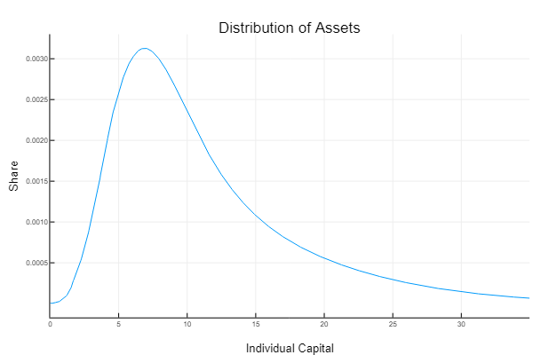
Interestingly, it does not appear that the addition of aggregate shocks leads to a considerable improvement in the model’s performance. The aggregate savings rate increases a bit, but the distribution of assets is still very similar to what you generate in a basic Aiyagari type model. To get a more realistic distribution, KS add ex-ante heterogeneity to their agents. Rather than having agents with identical expected utility functions, they allow agents to have different discount rates, which leads to different propensities to save.

Long-Run Distribution

References

Per Krusell & Anthony A. Smith & Jr., 1998. “Income and Wealth Heterogeneity in the Macroeconomy,” Journal of Political Economy, University of Chicago Press, vol. 106(5), pages 867-896, October.
S. Rao Aiyagari, 1994. “Uninsured Idiosyncratic Risk and Aggregate Saving,” The Quarterly Journal of Economics, Oxford University Press, vol. 109(3), pages 659-684.
Ellen R. McGrattan, 1993. “Solving the stochastic growth model with a finite element method,” Staff Report 164, Federal Reserve Bank of Minneapolis.
Young, Eric R., 2010. “Solving the incomplete markets model with aggregate uncertainty using the Krusell-Smith algorithm and non-stochastic simulations,” Journal of Economic Dynamics and Control, Elsevier, vol. 34(1), pages 36-41, January.

One thought on “Heterogeneous Agents with Aggregate Risk – Krusell/Smith”

someone says:

January 8, 2022 at 12:02 am

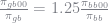
In the published version of paper condition :
πbg00 = 1.25 * πbb00

πgb00 = 0.75 * πgg00

has been replaced by
Pi_{gb00}*Pi_{gb}^{-1}= 1.25 Pi_{bb00}*Pi_{bb}^{-1}
Pi_{bg00}*Pi_{bg}^{-1}= 0.75 Pi_{gg00}*Pi_{gg}^{-1}

LikeLike