Heterogeneous Agents – Aiyagari

Many important questions in economics require us to consider heterogeneous agent models. For instance, the standard representative agent model could not be used to study the distribution of wealth because, by definition, a single agent has all of the wealth. Possibly the most important paper in this literature is S. Rao Aiyagari’s 1994 paper “Uninsured Idiosyncratic Risk and Aggregate Saving”. Aiyagari considered an economy where all the agents were ex ante identical, but due to a random income process were ex post heterogeneous. Additionally, he considered agents that were borrowing constrained so that they would be incentivized to increase savings for precautionary reasons. The following code replicates some results from Aiygari’s original paper and can be extended to replicate all of his results. For the interested reader, Aiyagari’s 1993 paper (of the same name) has additional results and elaborates further on the algorithm that he used.

The Model

The defining characteristic of the Aiyagari model is that there is uninsured idiosyncratic risk. This risk manifests itself as a shock to each consumer’s income process. For instance, this shock could determine whether or not a consumer is employed or how many hours they can work in a given period. The agent’s can invest in a single-period, risk-free bond. Importantly, markets are not complete, so the agents cannot perfectly insure their risks. The consumer’s problem is then given by

$\displaystyle E_0 \left\{ \sum_t \beta^t U(c_t)\right\}\\ \text{ s.t }c_t + a_{t+1} = w l_t + (1+r) a_t$

It is assumed that consumers are all identical ex-ante, but because they receive different shocks to their income, they will be different ex-post. Utility is generally given by

$\displaystyle U(c_t) = \frac{c_t^{1-\mu} - 1}{1-\mu}$

Aiyagari uses this functional form with various values for $\mu$ , (he considers $\mu \in \{1.0, 3.0, 5.0 \}$ ). Both $r$ and $w$ will be fixed in equilibrium at the stationary distribution and $a_t$ will be a control variable for the agent. Therefore, the idiosyncratic shocks will come from $l_t$ . It is assumed that $l_t$ follows the following autoregressive process

$\displaystyle \ln l_t = \rho \ln l_{t-1} + \sigma (1 - \rho^2)^{\frac{1}{2}} \epsilon_t$

where $\epsilon_t \sim \mathcal{N}(0,1)$ . The researcher might be interested in having labor that is supplied endogenously. In that case, $l_t$ becomes a control variable and the random shocks would come from some random $u_t$ that multiplies $w l_t$ . Production in this economy will take the standard Cobb-Douglas form

$\displaystyle y_t = \bar{k}^{\theta} \bar{l}^{1-\theta}$

where $\bar{k}$ and $\bar{l}$ denote the average capital and labor supplied by all agents. Note that there is no aggregate risk, e.g. a random TFP parameter $A_t$ on production, so if we are in equilibrium at the stationary distribution then $\bar{k}$ and $\bar{l}$ are fixed. As you will see below, the process for $l_t$ will be chosen so that $\bar{l} = 1.0$ and so production will take on the very simple form $\bar{k}^{\theta}$ .

The consumers are assumed to be borrowing constrained. Aiyagari denotes this constraint by

$\displaystyle \varphi = \min\left\{b, \frac{w l_{\min}}{r}\right\}$

Here $b$ is some arbitrary constraint that the researcher imposes on the agents. For instance, in the calculations below, we will assume that $b = 0.0$ . This means that agents cannot borrow, they can only save. However, if the researcher wants to allow for some positive amount of borrowing then they can choose $b > 0$ . The second term is deemed the “natural borrowing limit”. Here $w l_{\min}$ represents the lowest shock to income a consumer can receive. Consider an agent’s present discounted value of all future earnings, given that they get the bad shock in all periods. This is given by

$\displaystyle P_0 = \sum_{t=1}^{\infty} \frac{w l_{\min}}{(1+r)^{t+1}} = \frac{1}{1+r}\frac{w l_{\min}}{1 - \frac{1}{1+r}} = \frac{w l_{\min}}{r}$

This is the maximum amount a consumer could payback given that they received a series of bad shocks. Because an agent could never guarantee that they could payback more than this amount, it is the most that will be lent to them. Thus, it is the “natural borrowing limit” and we impose that $a_t \geq - \varphi$ . With this set-up, we can now turn to solving the model.

Solving the Model

After all of that discussion on the borrowing limit, Aiyagari uses a transformation of the model to effectively remove the limit. Rather than using $a_t$ as the state variable and $c_t$ as the control variable, Aiyagari defines the control variable

$\displaystyle \hat{a}_t = a_t + \varphi$

and the state variable

$\displaystyle z_t = w l_t + (1+r) \hat{a}_t - r \varphi$

We can think of $z_t$ as being the total amount of resources available to the consumer. This is because $z_t$ is equivalent to $w l_t + (1 + r) a_t + \varphi$ , so the most an agent can consume is their income plus their wealth plus the borrowing constraint. Now the control variable is constrained to be greater than or equal to zero, similar to capital in the standard growth model. Notice that the agent’s choice will be conditional on $z_t$ , and so $l_t$ will not matter once we know $z_t$ . This is important because we no longer need to treat $l_t$ as a state variable. This is important for solving the model and was completely lost on me the first three times I read the paper.

The consumer’s problem will now be written as

$\displaystyle E_0 \sum_t \beta^t\left[\frac{(z_t - \hat{a}_{t+1})^{1-\mu} - 1}{1-\mu} + \frac{\zeta}{3}\min\{\hat{a}_{t+1},0\}^3 \right]\\ \text{s.t. } z_t = w l_t + (1+r)\hat{a}_t - r\varphi,\ \forall t$

The term 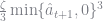$\frac{\zeta}{3}\min\{\hat{a}_{t+1},0\}^3$ is meant to account for the fact that $\hat{a}_t$ needs to be greater than 0. As $\zeta \to \infty$ the solution to this problem coincides with the solution when $\hat{a}_t \geq 0$ . Importantly though, this formulation is smooth and so is easier to solve. More on this below.

Following Aiyagari, we will use the following parameters

# Model Primitives
β = 0.96
δ = 0.08
α = 0.36
μ = 5.0 # μ ∈ {1,3,5}

To solve this model we need a finite representation for the process $\ln l_t$ and the decision rule $\hat{a_t}(z_t, w, r)$ . For the stochastic process I follow Aiyagari and approximate the $AR(1)$ process with a Markov Chain using Tauchen’s method. For the decision rule, I use the Finite Element Method.

Tauchen’s Method

Tauchen (1986) proposed a method of approximating an $AR(1)$ process using a Markov chain. The first thing that we need to do is create a grid over $\ln l_t$ . To determine the maximum and minimum values of your grid, Tauchen recommends using $3$ standard deviations of the process around its steady state. In this case, the variance of our process is given by $\sigma^2$ and so we will use the grid points $\{- 3 \sigma, -2 \sigma, -\sigma, 0.0, \sigma, 2 \sigma, 3 \sigma\}$ . The following code creates a grid for each state. I have set-up the code to generalize to multiple state variables (for instance, Business Cycle Accounting uses four state variables), but only one is needed to replicate Aiyagari.

using Cubature
N = 7 # Number of grid points
m = 3 # Number of standard deviations
σ = 0.2 # σ ∈ {0.2, 0.4}
ρ = 0.6 # ρ ∈ {0.0, 0.3, 0.6, 0.9}
Σ = σ^2*sqrt(1-ρ^2)^2# Correlation Matrix
Σy = σ # Standard Deviation
ivΣ = 1/Σ
# Calculate Grid Values and Steps
maxy = m*Σy # Three standard deviations high
miny = -m*Σy # Three standard deviations low
ys = collect(linspace(miny, maxy, N)) # Vector of values
step = ys[end]/(N-1) # Step size
ys

7-element Array{Float64,1}:
 -0.6
 -0.4
 -0.2
  0.0
  0.2
  0.4
  0.6

Next, we need to calculate the probability in each interval of our grid. Note that $\ln l_t - \rho \ln l_{t-1} = \epsilon_t \sim \mathcal{N}\left(0, \sigma^2(1-\rho^2)\right)$ . So to calculate the transition probabilities from one state to the next, we can calculate this difference and then integrate the normal distribution between those grid points.


# Calculate Markov Matrix

P = zeros(N, N);
for j = 1:N
    μ = ρ*ys[j]
    for l = 1:N
        lowX = ys[l] - μ - step
        l == 1 && (lowX = ys[l] - μ - step - 100.0)
        highX = ys[l] - μ + step
        l == N && (highX = ys[l] - μ + step + 100.0)
        (val,err) = hcubature(x -> exp(-.5*x'*ivΣ*x)[1], lowX, highX,
        reltol=1e-4, abstol=0, maxevals=0)
        P[j,l] = (val ./ sqrt(2 *pi * Σ))
    end
end

P = P ./ sum(P, 2)

  0.467838 seconds (527.03 k allocations: 22.734 MB, 1.22% gc time)

7×7 Array{Float64,2}:
 0.190787     0.455383     0.301749   …  0.0020016  1.84984e-5   3.82913e-8 
 0.0520813    0.301749     0.455383      0.0164242  0.000367205  1.87299e-6 
 0.00877448   0.12152      0.419444      0.0802333  0.00427914   5.33123e-5 
 0.000889025  0.0295073    0.235589      0.235589   0.0295073    0.000889025
 5.33123e-5   0.00427914   0.0802333     0.419444   0.12152      0.00877448 
 1.87299e-6   0.000367205  0.0164242  …  0.455383   0.301749     0.0520813  
 3.82913e-8   1.84984e-5   0.0020016     0.301749   0.455383     0.190787

In the above code, I use the Cubature package to carry out the integration. You could also using Gauss-Hermite quadrature to evaluate this integral as well. The difference in run-time doesn’t matter when we use a coarse grid.

This defines the Markov transition matrix that approximates our original AR(1) process. This allows us to perform our calculations on a single continuous state variable (in this case capital) and one discrete state variable (the income process), which will lead to simpler calculations. Aiyagari renomalizes the income process so that the average amount of labor supplied is equal to $1$ at the stationary distribution. To do this, he finds the stationary distribution of the Markov process and the renormalizes it to be equal to $1$ .

statdst = inv((eye(N) - P + ones(N,N))')*ones(N)
El = dot(exp(ys)',statdst)
L = exp(ys)/El

Finite Element Method

There are a number of different ways to solve for the consumer’s policy function. Probably the most commonly used are value function or policy iteration. Because those have been done elsewhere, I will use the Finite Element Method instead. I won’t go into the details of implementing the Finite Element Method here, but instead will only discuss its application to this problem. A more general treatment of the method can be found in Ellen McGrattan’s 1993 paper.

The first-order conditions of our approximate problem are given by

$\displaystyle (z_t - \hat{a}_{t+1})^{-\mu} - \zeta \min\{\hat{a}_{t+1},0\}^2 = (1+r)\beta \sum_{s^{\prime}}\pi_{s^{\prime}} (z_{t+1} - \hat{a}_{t+2})^{-\mu}$

We want to approximate the optimal savings function using a piecewise linear function, that is

$\displaystyle \hat{a}(z, s) = \sum_i \phi(z)_{i} \alpha_{i,s}$

Here $\phi(z)_{i\in I}$ is the “hat” basis function and the $\alpha_{i,s}$ are the values of our approximation at a predetermined set of $I$ nodes. The hat basis function has the following form

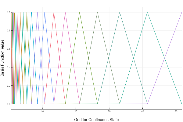
Notice that they range from 0 to 1, and only two basis functions are non-zero between any two points on our grid (our grid points are located where the basis functions become zero). Also notice that our grid over the continuous state does not have to be evenly spaced. In this example, we have placed more points near 0 as this is where the kink is in the savings policy function. The coefficients for our linear approximation will be equal to the policy function at each point on our grid, and for points not falling on our grid, we will linearly approximate between the neighboring coefficients.

We need to choose values for the coefficients that generates a good approximation of our policy function, i.e. the average error in our Euler Equation will be small. To do this, I use the method of weighted residuals. Define the residual of the Euler Equation as

$\displaystyle R(z, s, \alpha) = (z - \hat{a}^{\prime})^{-\mu} - \zeta \min\{\hat{a}^{\prime},0\}^2 - (1+r)\beta \sum_{s^{\prime}}\pi_{s, s^{\prime}} (z^{\prime} - \hat{a}^{\prime\prime})^{-\mu}$

If we had the true policy function, this residual would be zero everywhere. We unfortunately do not have the true policy function, so we are going to try and minimize a special weighted integral of this residual equation. Specifically, we will choose our $\alpha_{i,s}$ so that for each state $s$

$\displaystyle \int R(z, s, \alpha)\phi(z)_i dz = 0,\ \forall i = 1,...,K$

where $K$ is our grid size. This is a system of $K \times S$ equations in the same number of unknowns. The $phi(z)_i$ are our “hat” basis functions. One doesn’t need to use this weight function, which is the Galerkin method, but it has nice properties. See McGrattan’s paper for the details.

As always, we start with a custom type which we will use to store the model parameters as well as the transition matrix, the grids, and the coefficients for our interpolation.

# Interpolating Object
type GalerkinObj
    β::Float64
    δ::Float64
    α::Float64
    ψ::Float64
    μ::Float64
    ϕ::Float64
    w::Float64
    r::Float64
    ζ::Float64
    P::Array{Float64, 2}
    states::Array{Float64,1}
    θs::Array{Float64, 2}
    grid::Array{Float64, 1}
    
    function GalerkinObj(β, δ, α, ψ, μ, ϕ, w, r, ζ, P, states, grid)
        return new(β, δ, α, ψ, μ, ϕ, w, r, ζ, P, states, zeros(length(states), length(grid)), grid)
    end
end

We now define a few helpful routines, taking advantage of Julia’s multiple dispatch. The first routine that we define simply takes an input $k$ for the continuous state and an input $s$ for the discrete state, and then calculates the interpolated value given the current set of coefficients. The way it does this is by using a binary search to find where $k$ falls in our grid and then returns an interpolated value using the coefficients at the two closest grid points. The next two routines calculate the derivatives of our linear approximation with respect to a coefficient $\alpha_{i,s}$ (in the first routine) and with respect to the continuous state variable $k$ (in the second routine). We will be using these derivatives to solve the weighted residuals equation.


# Interpolate for specific state
function(itp::GalerkinObj)(k::Float64, s::Int)
    g = itp.grid
    k >= g[end] && return itp.θs[s, end] * k/g[end]
    g[1] = g[end]) & (d == length(itp.grid)) && return k/g[end]
    (g[1] = g[end] && return itp.θs[s, end] / g[end]
    g[1] < k && return 0.0 #* k/g[1]
    lb = searchsortedlast(itp.grid, k)
    ub = lb + 1
    return -itp.θs[s, lb] * 1.0/(g[ub] - g[lb]) + itp.θs[s,ub] * 1.0 /(g[ub] - g[lb])
end

To define the relevant grids, it helps to identify the minimum and maximum sustainable cash-in-hand. The minimum cash-in-hand that an agent can have is the lowest wage in the lowest productivity state. The lowest wage occurs when the highest interest rate occurs, which is equal to the time value of consumption. The largest sustainable cash-in-hand occurs when the capital stock is at its maximum sustainable value, i.e. when production perfectly offsets depreciation. I use these values as the lower and upper bound on my grid, and then use a nonlinear transformation to place more points near the origin.

lmin = L[1]
# Implied minimum wage and cash on hand
rT = 1/β-1
wmin = (1-α)*(α/(rT + δ))^(α/(1-α)) # L/K evaluated when r = rT
zmin = wmin*lmin
# Implied maximum capital and cash on hand
kmax = δ^(1/((α-1)))
zmax = kmax^α + (1-δ)*kmax
# Initial guess for interest rate and wages
rav = rT*0.72
wav = (1-α)*(α/(rav + δ))^(α/(1-α))
# Grid over cash-on-hand
zGrid = convert(Array, collect(linspace(zmin^(1/50), zmax^(1/50), 20))).^50;
# Maximum amount an agent can save is just the cash-in-hand
maxa = zGrid'

Using these values, we initialize our custom type.

go = GalerkinObj(β, δ, α, ψ, μ, 0.0, wav, rav, 0.0, P, L, zGrid);

We need to translate the residual equation into a function. No surprises here, the below function is a direct translation of the residual equation into code.

function R_all(z::Float64, s::Int64, â::GalerkinObj)
β, δ, α, ψ, μ, ϕ, w, r, ζ, P = â.β, â.δ, â.α, â.ψ, â.μ, â.ϕ, â.w, â.r, â.ζ, â.P
    l = â.states
    â′ = â(z, s)
    rhs = (z - â′ )^(-μ) - ζ * min(â′, ϕ)^2
    lhs = 0.0
    for j in eachindex( l )
        z′s = w*l[j] + (1.0+r)*â′ - r*ϕ
        lhs += (z′s - â(z′s, j))^-μ * P[s, j]
    end
    lhs = (1.0 + r)*β*lhs
    return rhs - lhs
end

It will also be helpful to define the derivative of the residual equation with respect to an arbitrary coefficient $\alpha_{i,s}$ (in the below function, i = d and s = d2). We will be using Newton’s Method to solve the system of weighted residual equations, and so we will need to be able to calculate this derivative at arbitrary points. The only part below that is tricky is evaluating the derivative of $\hat{a}(z^{\prime}, s)$ with respect to a given coefficient. The coefficients can change its value either directly or by changing $z^{\prime} = w l + (1 + r)\hat{a}(z, s)$ . We therefore need to use a total derivative, i.e.

$\displaystyle \frac{d \hat{a}(z^{\prime}, s)}{d \alpha_{i,s}} = \frac{\partial \hat{a}(z^{\prime}, s)}{\partial \alpha_{i,s}} + \frac{\partial \hat{a}(z^{\prime}, s)}{\partial z^{\prime}}\frac{\partial z^{\prime}}{\partial \alpha_{i,s}}$

function R′_all(d::Int64, d2::Int64, z::Float64, s::Int64, â::GalerkinObj)
    β, δ, α, ψ, μ, ϕ, w, r, ζ, P = â.β, â.δ, â.α, â.ψ, â.μ, â.ϕ, â.w, â.r, â.ζ, â.P
    â_d = â(d, z, d2)
    l = â.states
    â′ = â(z, s)
    rhs = μ*(z - â′ )^(-μ-1.0)*â_d*(d2==s) - ζ * 2.0 * min(â′, ϕ)*â_d*(d2==s)
    lhs = 0.0
    if d2 == s
        for j in eachindex( l )
            z′s = w*l[j] + (1.0+r)*â′ - r*ϕ
            lhs += -μ*(z′s - â(z′s, j))^(-μ-1.0)*((1.0+r)*(â_d - â(z′s, j, 1)*â_d) - â(d, z′s, j)*(s==j)) * P[s, j]
        end
    else
        z′s = w*l[d2] + (1.0+r)*â′ - r*ϕ
        lhs = -μ*(z′s - â(z′s, d2))^(-μ-1.0)*( - â(d, z′s, d2) ) * P[s, d2]
    end
    lhs = (1.0 + r)*β*lhs
    return rhs - lhs
end

This last function we need calculates the weighted residual equations and then uses Newton’s Method to set the system of equations as close to zero as possible. I set the tolerance to $10^{-5}$ , although Newton’s Method converges so fast that you could use a higher tolerance without much additional run-time.

function weightedResidual(go::GalerkinObj, N::Int64)
    nodes, weights = gausslegendre(N)
    rescl = zeros(length(nodes))
    Gθ = zeros(length(go.θs), length(go.θs))
    res = zeros(length(go.θs))
    g = vcat([go.grid[1]], go.grid, [go.grid[end]])
    eps = vec(go.θs)
    count = 1
    while (maximum(abs(eps)) > 1e-5)*(100 > count)
        count += 1
        # Reset Values to zero
        for i = 1:length(res)
            res[i] = 0.0
            for j = 1:length(res)
                Gθ[i,j] = 0.0
            end
        end
        for i = 3:length(g)
            for j = 1:length(nodes)
                rescl[j] = (nodes[j] + 1.0)*(g[i]-g[i-2])/2.0 + g[i-2]
            end
            for s = 1:length(go.states)
                idx1 = length(go.states)*(i-3) + s
                for j = 1:length(rescl)
                    newweight = ifelse( g[i-1] < rescl[j],
                    (rescl[j] - g[i-2])/(g[i-1] - g[i-2])  ,
                    (g[i] - rescl[j])/(g[i] - g[i-1])
                    ) * weights[j] * (g[i]-g[i-2])/2.0
                    res[idx1] += R_all(rescl[j], s, go) * newweight
                    for gs = 1:length(go.states)
                        for gp = 1:length(go.grid)
                        idx2 = length(go.states)*(gp-1) + gs
                        Gθ[idx1, idx2] += R′_all(gp, gs, rescl[j], s, go) * newweight
                        end
                    end
                end
            end
        end
        eps = -Gθ\res
        for i = 1:length(go.θs)
        go.θs[i] += eps[i]
        end
    end
    @show maximum(abs(eps))
    return nothing
end

I set $\zeta = 100,000$ . This is a bit of overkill, as a lower value generates a close approximation as well. Remember that as $\zeta \to \infty$ , the smooth approximation converges to the one with a kink. I set my guess to $0.97$ times the current cash-in-hand for every discrete state. This closely approximates the true policy function for large values of $z$ and so works well in practice.

go.ζ = 100000.0
go.θs = maxa*0.97.*ones(ys);
@time weightedResidual(go, 9)

maximum(abs(eps)) = 2.802889423022742e-6
  3.282654 seconds (483 allocations: 8.643 MB, 0.14% gc time)

The policy function generated by this code is identical to that reported in Aiyagari 1993.

Calculating the Stationary Distribution

The final step in solving the Aiyagari model is calculating the stationary distribution. Finding the stationary distribution involves solving for the interest rate and wage such that next periods average capital is the same as the current periods. The first hurdle is solving for the average capital holdings given a fixed interest rate. Aiyagari used the fact that the capital distribution is ergodic and calculated the average asset holdings from a long time series for a single agent. In subsequent studies, researchers have instead simulated short time series for many agents and then calculated average asset holdings across all agents in the last few periods. Both of these methods work and are fairly robust, however they aren’t very efficient. Young (2010) proposed discretizing the asset distribution and then calculating a transition matrix for this discrete distribution using the known transition probabilities and the agent’s policy function. Violante has a good discussion of this method in his course notes here.

The function below takes our policy function object $\hat{a}$ and a fine grid over capital (I choose 500 points between -0.1, because the policy function isn’t precisely zero at he lower bound, and 200.0) and then uses the transition matrix $P$ to generate the transition dynamics. It is highly unlikely that our policy function will prescribe asset holdings next period that are on our discrete grid, so when assets fall in between two grid points we do an inverse interpolation. That is, we distribution the weight of these assets to the two grid points, placing more weight on the grid point that is closest. Given a transition matrix, we can then simply calculate the stationary distribution using the following formula

$\displaystyle \lambda =\left(I - \Phi + \iota_{M\times M} \right)^{-1}\iota_{M \times 1}$

where $\iota_{M\times M}$ is a matrix of ones and $\iota_{M\times 1}$ is a vector of ones. $\Phi$ is our calculate transition matrix. Once we have the stationary distribution, we can simply multiply it by the asset grid (repeated as many times as the number of states there are) and sum up the values to get our average capital.


function calcStatDist(â::GalerkinObj, agrid)
P = â.P
r3 = â.r
w3 = â.w
Φ = zeros(size(P,1)*length(agrid), size(P,1)*length(agrid));
AM = size(Φ,1)
M = length(agrid)
    for i = 1:AM
        k = div(i-1, M) + 1
        a1 = ifelse(mod(i, M) == 0, M, mod(i, M))
        a′ = â(agrid[a1]*(1+r3) + w3*L[k], k)
        indxL = searchsortedlast(agrid, a′)
        indxH = indxL + 1
        w1 = (agrid[indxH] - a′)/(agrid[indxH] - agrid[indxL])
        w2 = (a′ - agrid[indxL])/(agrid[indxH] - agrid[indxL])
        for j = 1:size(P,1)
            Φ[i,M*(j-1) + indxL] = P[k, j] * w1
            Φ[i,M*(j-1) + indxH] = P[k, j] * w2
        end
    end
Φ = Φ./sum(Φ,2);
statDist = (eye(M*size(P,1)) - Φ + ones(M*size(P,1),M*size(P,1)))'\ones(M*size(P,1))
dot(statDist, repeat(agrid, outer = size(P,1)))::Float64
end

Once we have determined our average capital, we need to search over values of $r$ to find the one that generates a stationary distribution. Remember that $w$ is fixed conditional on $r$ , so we are searching over a single variable to find a fixed point. Aiyagari proposed using a bisection method to find the interest rate that solves our problem and that is what I have implemented below. It is slow but robust.

To find the correct interest rate, we will compare the average capital implied by our transition matrix and compare it to the capital that generates our current guess of $r$ . Given an interest rate $r$ we can calculate the capital holdings that are commensurate with is by

$\displaystyle K = \left( \frac{r + \delta}{\alpha} \right)^{-\frac{1}{1-\alpha}}$

If our policy function generates average holdings above this, we know that the interest rate is too high, i.e. agents are over-investing, and we adjust it downwards. If our policy function generates a lower capital stock then agents are under-investing and we adjust the interest rate upwards. The bisection method continuously updates the lower and upper bounds of our interest rate depending on whether our previous guess was too low or two high and will eventually converge to the stationary interest rate.


function bisection(go::GalerkinObj, agrid::Array{Float64,1})
    α = go.α
    δ = go.δ
    rT = 1.0 - 1.0\go.β
    r3 = rT*0.72 # Initial Guess
    r2 = rT # Upper bound
    r1 = 0.0 # Lower Bound
    eps = 1.0; count = 0
    while(eps > 1e-5)*(5 > count)
        rtmp = (r1 + r2)/2
        eps = abs(rtmp - r3)
        r3 = deepcopy(rtmp)
        @show eps
        w3 = (1-α)*(α/(r3 + δ))^(α/(1-α))
        maxa = max((1+r3)*zGrid' .+ w3*L,0)

        newP2 =  findRoot(vec(αs2), r3, w3)
        αs2 = reshape(newP2, size(L,1), length(zGrid))
        â = GalerkinObj(αs2, zGrid);
        stD, as  = calcStatDist(â, P, r3, w3, Max = 200.0, N = 500)
        agrid = collect(linspace(-0.1, 200, 500));
        a′ = vcat([â(a)' for a in agrid]...);
        e = (1.0 - ψ*((1+r3)*agrid .- a′)./(L'*w3))/(1+ψ);
        tmp = reshape(stD, Int(length(stD)/size(P,1)), size(P,1))
        Lss = sum(tmp.*e)
        K3 = ((r3+δ)/α)^(-1/(1-α))*Lss
        as > K3 && (r2 = r3)
        K3 > as && (r1 = r3)
        count += 1
    end
    return nothing

end

@time bisection(go, agrid)

maximum(abs(eps)) = 3.809819676979794e-6
maximum(abs(eps)) = 8.95310406449911e-6
maximum(abs(eps)) = 3.7637412435255835e-8
maximum(abs(eps)) = 8.684272846885449e-8
maximum(abs(eps)) = 4.667653538520587e-6
maximum(abs(eps)) = 5.434474939187872e-8
maximum(abs(eps)) = 3.933242153661582e-9
maximum(abs(eps)) = 2.4705718111657407e-10
maximum(abs(eps)) = 3.95137873051283e-6
maximum(abs(eps)) = 9.838429366693355e-7
maximum(abs(eps)) = 2.457911398865253e-7
maximum(abs(eps)) = 6.146862346294397e-8
 44.151404 seconds (621.98 k allocations: 8.789 GB, 16.62% gc time)

The resulting interest rate for capital is very close to what Aiyagari originally calculated (see Table II in Aiyagari (1994) for the case when $\mu = 5$ and $\rho = 0.6$ ). We can always get a more accurate approximation by using a finer grid for the capital distribution or our policy function, a lower tolerance in our Newton’s Method, or increasing the number of quadrature nodes.


go.r

0.035986328125000036

References

S. Rao Aiyagari, 1994. “Uninsured Idiosyncratic Risk and Aggregate Saving,” The Quarterly Journal of Economics, Oxford University Press, vol. 109(3), pages 659-684.
Ellen R. McGrattan, 1993. “Solving the stochastic growth model with a finite element method,” Staff Report 164, Federal Reserve Bank of Minneapolis.
Young, Eric R., 2010. “Solving the incomplete markets model with aggregate uncertainty using the Krusell-Smith algorithm and non-stochastic simulations,” Journal of Economic Dynamics and Control, Elsevier, vol. 34(1), pages 36-41, January.

The Model

Solving the Model

Tauchen’s Method

Finite Element Method

Calculating the Stationary Distribution

References

Share this:

Like this:

Leave a Reply Cancel reply