Expectation-Maximization Algorithm

I want to discuss two papers which deal with unobserved heterogeneity in dynamic discrete choice models, Arcidiacono & Jones (2003) and Arcidiacono & Miller (2011), but first it will help to review the estimation routine that they are based on, the expectation-maximization (EM) algorithm. Kenneth Train provides a comprehensive overview of these methods in his book “Discrete Choice Methods with Simulation” and I would highly recommend reading section 14.2 to get an understanding of why the algorithm works. One of the examples that I use below is based on his paper “A Recursive Estimation for Random Coefficients Model“, the data for which is provided in the mlogit package in R.

The EM algorithm is a quintessential example of how generalizing a problem can sometimes make it simpler. First, consider standard maximum likelihood estimation. We want to find the parameter estimates that maximize the log-likelihood of generating our sample, i.e.

$\hat{\theta} = \text{argmax}\ \ln P(X\ \vert\ \theta) \\$

Let $z$ be some data that we wish we had and assume that it is distributed according to $f(z\ \vert\ \theta)$ (it is necessary for us to explicitly define this distribution during estimation). The log-likelihood can be written as

$\ln P(X\ \vert\ \theta) = \ln \int P(X\ \vert\ z, \theta) f(z\ \vert\ \theta)dz$

If we had access to the missing data then a reasonable estimation procedure would be to maximize the joint log-likelihood of the sample and the missing data. Of course, the missing data is just that, missing. Because we know $f(z\ \vert\ \theta)$ and $P(X\ \vert\ z, \theta)$ we can integrate out the $z$ conditional on $x$ and maximize the conditional expected value of joint log-likelihood. More explicitly, Bayes Theorem gives

$h(z\ \vert\ X, \theta) = \frac{P(X\ \vert\ z, \theta) f(z\ \vert\ \theta)}{P(X\ \vert\ \theta)}$

The joint likelihood is given by

$LL(\theta\ \vert\ X, z) = \ln P(X\ \vert\ z, \theta) f(z\ \vert\ \theta)$

so the conditional expectation is given by

$\mathcal{E}(\theta) = \int h(z\ \vert\ X, \theta) \ln \left( P(X\ \vert\ z, \theta) f(z\ \vert\ \theta) \right) dz$

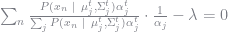
It turns out that the estimator which maximizes this expected log-likelihood will also maximize our original log-likelihood. Furthermore, there is a simple iterative process which is guaranteed to converge to a local maximum of the likelihood function. Instead of maximizing $\mathcal{E}(\theta)$ directly, consider starting with a parameter guess $\theta^0$ and maximizing

$\mathcal{E}(\theta\ \vert\ \theta^0) = \int h(z\ \vert\ X, \theta^0) \ln \left( P(X\ \vert\ z, \theta) f(z\ \vert\ \theta) \right) dz$

We can then take the parameter estimate $\theta^1$ that maximizes this expression and maximize $\mathcal{E}(\theta\ \vert\ \theta^1)$ . Under fairly general conditions this process is guaranteed to monotonically increase the likelihood function and to converge to a local maximum (again, for a demonstration of this claim see section 14.2 of Train’s book). This has all been very abstract, so to make it concrete I go over the estimation in Train’s paper “A Recursive Estimation for Random Coefficients Model”.

Replicating Train’s Analysis

In this paper, Train is modeling the behavior of agents choosing between four electricity providers. He parameterizes the utility from choice $j$ as

$U_{ij} = x_{j}^{\prime}\beta_{i} + \epsilon_{ij}$

Train’s data is setup in a wide format. The second column gives the agent’s ID and the first column records the agent’s choice in situation $t$ . The next four columns provide the first element of $x_{ijt}$ for the four choices, the next provide the second element for the four choice, and so on. I import and convert the raw data to a matrix using the below code.

using DataFrames
using DataFramesMeta

electricity = readtable("[path]/Electricity.csv", header = true, separator = ',');

dataMat = convert(Array, electricity)
ids = unique(dataMat[:,2])

He parameterizes the utility from choice $j$ as

$U_{ij} = x_{j}^{\prime}\beta_{i} + \epsilon_{ij}$

where $\beta_{i}$ is a random coefficient that is distributed normally and $\epsilon_{ij}$ is a random error term that is distributed Type 1 extreme value. As always, we can integrate out the error terms to get a choice probability of

$L_{ij} = \frac{\exp(x_j^{\prime}\beta_i)}{\sum_k \exp(x_k^{\prime}\beta_i)}$

The below function takes a vector of the $x_{ijt}$ , the choice $y_{ijt}$ and a vector $\beta_i$ (or a matrix of $\beta_i$ ‘s) and returns the choice probabilities.

function L(obs_n, choice_n, β_n)
    choiceCols = collect(2+choice_n:4:26)
    base = obs_n[choiceCols]' * β_n'
    denom = zeros(obs_n[choiceCols]' * β_n' )
    for j = 1:4
        optCols = collect(2+j:4:26)
        denom .+= exp( obs_n[optCols]' * β_n'  .- base )
    end    

    return 1 ./ denom
end

Each agent is observed in $T$ choice situations, so we need to add a new index for each situation. Let this index be given by $t$ and let $L_{ijt}(y_{ijt}\ \vert\ x_{jt}, \beta_i)$ be the probability of their observed choice $y_{ijt}$ in situation $t$ . The likelihood of observing their choices $y = (y_{ij1}, y_{ij2}, ..., y_{ijT})$ is given by

$P(y\ \vert\ x_{jt}, \beta_i, \theta) = \prod_t L_{ijt}(y_{ijt}\ \vert\ x_{jt}, \beta_i, \theta)$

In this case, our missing data $z$ is the set of $\beta_i$ for each agent. By assumption, $\beta_i \sim N(\mu, \Sigma)$ , meaning that $\theta = (\mu, \Sigma)$ . Let $\phi(\beta_i\ \vert\ \mu, \Sigma)$ be the pdf of the normal distribution. Then $h(z\ \vert\ y, \theta^t)$ is given by

$h(\beta_i\ \vert\ y, \mu^t, \Sigma^t) = \frac{P(y\ \vert\ x_{jt}, \beta_i, \mu^t, \Sigma^t)}{P(y\ \vert\ x_{jt}, \mu^t, \Sigma^t)}\phi(\beta_i\ \vert\ \mu^t, \Sigma^t)$

where

$P(y\ \vert\ x_{jt}, \mu^t, \Sigma^t) = \int P(y\ \vert\ x_{jt}, \beta_i, \mu^t, \Sigma^t)\phi(\beta_i\ \vert\ \mu^t, \Sigma^t)d\beta_i$

Note that we can calculate $P(y\ \vert\ x_{jt}, \beta_i, \mu^t, \Sigma^t)$ from the data and we can draw from the density $\phi(\beta_i\ \vert\ \mu^t, \Sigma^t)$ easily enough with most programming languages. The only difficulty is calculating $P(y\ \vert\ x_{jt}, \mu^t, \Sigma^t)$ . Train resolves this by using simulation. We can approximate the above integral numerically by

$P(y\ \vert\ x_{jt}, \mu^t, \Sigma^t) = \int P(y\ \vert\ x_{jt}, \beta_i, \mu^t, \Sigma^t)\phi(\beta_i\ \vert\ \mu^t, \Sigma^t)d\beta_i \approx \frac{1}{R} \sum_r P(y\ \vert\ x_{jt}, \beta_{ir}, \mu^t, \Sigma^t)$

where $\beta_{ir}$ are randomly samples from the pdf $\phi(\beta_i\ \vert\ \mu^t, \Sigma^t)$ . Train doesn’t actually use a random sample in his estimation and instead uses random Halton sequences as they provide a lower sampling variance for his parameter estimates. While I won’t go into the details of Halton sequences (or randomized Halton sequences), the below code will generate the required draws. If you are interested in how this code was generated and the underlying rational for using Halton draws, you should read section 9.3.3 of Train’s book. Following Train I sample 200 $\beta_i$ s for each agent. Note that if $c$ is the Cholesky factor of $\Sigma$ and $h$ is distributed standard normal, then $\beta_i = \mu + c \cdot h$ is distributed $N(\mu, \Sigma)$ . I therefore create standard normal Halton draws and then transform them later.

using StatsFuns

R = 200 # Number of sampled draws

function Halton(i = 1, b = 3)
    f = 1 # value
    r = 0
    while i > 0
        f = f / b
        r = r + f * mod(i, b)
        i = floor(i/b)
    end
    return r
end

function HaltonDraws( k=6, n = 200, primeList = [3, 7, 13, 11, 2, 5])
    draws = zeros(n, k)

    myPrimes = primeList
    for j = 1:k
        draws[:,j] = [Halton(i, myPrimes[j]) for i = 100:100+n - 1]';
    end
    println(myPrimes)
    return draws
end

halt = HaltonDraws(6, R * length(ids))

srand(123456)

halt = mod( rand(size(halt)) .+ halt, 1 )

for i = 1:(R * length(ids))
    for j = 1:6
        halt[i,j] = norminvcdf(halt[i,j] )
    end
end

We start with an initial guess for the parameter estimates. I start with

b0 = [1.0 1.0 1.0 1.0 1.0 1.0]
W0 = eye(6)*10 + 5
c = chol(W0)
βs = []
ws = []

where b0 is the vector of means and W0 the covariance matrix for our normal distribution, and c is the Cholesky decomposition of W0. We can now create a sequence of draws for $\beta_i$ as

βnr = b0 .+ halt[200*(i-1)+1:200*i, :] * c

Our simulated likelihood for agent $i$ is then calculated as

tmpInd = find(dataMat[:,2] .== i)
obs = dataMat[ tmpInd ,:]

βnr = b0 .+ halt[R*(i-1)+1:R*i, :] * c
wnr = ones(R)

for t = 1:size(obs,1)-1
    sub = obs[t,:]
    Ls = L(sub, sub[1], βnr)
    wnr = wnr .* Ls'
end

P_y = mean(wnr)

(the astute reader will notice that we calculate the likelihood with $T-1$ observations. This is because Train holds out one observation for each agent to validate his results). In this example the expectation that we want to maximize is given by

$\mathcal{E}(\theta\ \vert\ \theta^t) = \sum_i \int \frac{P(y\ \vert\ x_{jt}, \beta_i, \mu^t, \Sigma^t)}{P(y\ \vert\ x_{jt}, \mu^t, \Sigma^t)}\phi(\beta_i\ \vert\ \mu^t, \Sigma^t) \ln \left( P(y\ \vert\ x_{jt}, \beta_i, \mu^t, \Sigma^t) \phi(\beta_i\ \vert\ \mu, \Sigma) \right) dz$

(where we have now summed over the $N$ agents). We also use simulation to approximate the expectation

$\mathcal{E}(\theta\ \vert\ \theta^t) \approx \sum_i\frac{1}{R}\sum_r \frac{P(y\ \vert\ x_{jt}, \beta_i, \mu^t, \Sigma^t)}{P(y\ \vert\ x_{jt}, \mu^t, \Sigma^t)} \ln \left( P(y\ \vert\ x_{jt}, \beta_i, \mu, \Sigma) \phi(\beta_i\ \vert\ \mu, \Sigma) \right)$

Note that $P(y\ \vert\ x_{jt}, \beta_i, \mu, \Sigma)$ does not depend on $\mu$ and $\Sigma$ , conditional on $\beta_i$ . Therefore, maximizing the above expression with regards to $\mu$ and $\Sigma$ is the same as maximizing

$\sum_i\frac{1}{R}\sum_r \frac{P(y\ \vert\ x_{jt}, \beta_i, \mu^t, \Sigma^t)}{P(y\ \vert\ x_{jt}, \mu^t, \Sigma^t)} \ln \phi(\beta_i\ \vert\ \mu, \Sigma)$

This maximization problem is simple to carry out, it is just the maximum likelihood estimator for a weighted normal distribution, i.e. the weighted mean and weighted covariance. Therefore

$\mu^{t+1} = \frac{1}{N}\sum_i\frac{1}{R}\sum_r w_{ir} \beta_{ir}$

and

$\Sigma^{t+1} = \frac{1}{N}\sum_i\frac{1}{R}\sum_r w_{ir} (\beta_{ir} - \mu^{t+1})(\beta_{ir} - \mu^{t+1})^{\prime}$

where

$w_{ir} = \frac{P(y\ \vert\ x_{jt}, \beta_i, \mu^t, \Sigma^t)}{P(y\ \vert\ x_{jt}, \mu^t, \Sigma^t)}$

My combined code for the EM algorithm is

@time while criter > .001
    c = chol(W0)
    βs = []
    ws = []

    for i = 1:length(ids)
        tmpInd = find(dataMat[:,2] .== i)
        obs = dataMat[ tmpInd ,:]

        βnr = b0 .+ halt[R*(i-1)+1:R*i, :] * c
        wnr = ones(R,1)

        for j = 1:size(obs,1)-1
            sub = obs[j,:]

            Ls = L(sub, sub[1], βnr)

            wnr = wnr .* Ls'
        end
        append!(βs, [βnr])
        append!(ws, wnr ./ mean(wnr) )

    end

    βs = vcat(βs...)
    b1 = sum(ws .* βs, 1) / (length(ids) * R)

    weightedW = zeros(6, 6)
    for k = 1:size(βs,1)
        BLAS.syr!('U', ws[k], (βs[k,:]' .- b1)'[:], weightedW)
    end

    W1 = Symmetric(weightedW / (length(ids) * R))

    criter = maximum([maximum(abs(b0 .- b1)./abs(b0)), maximum(abs(W1.-W0)./abs(W0))])

    b0 = b1
    W0 = W1

end
b0
W0

209.007623 seconds (1.00 G allocations: 139.476 GB, 26.76% gc time)
-0.937996  -0.221032  2.43001  1.84637  -8.83472  -8.97277

6×6 Symmetric{Float64,Array{Float64,2}}:
  0.283332   -0.0156035  0.983562  0.666749   2.42428   2.28836 
 -0.0156035   0.152333   0.248331  0.175803  -0.18654  -0.246001
  0.983562    0.248331   4.10506   2.55159    8.58359   7.94201 
  0.666749    0.175803   2.55159   2.30071    5.46891   4.82644 
  2.42428    -0.18654    8.58359   5.46891   28.2993   22.3985  
  2.28836    -0.246001   7.94201   4.82644   22.3985   22.5691

My results do not match Train’s precisely, but that is likely due to simulation variation. As you can see, the estimated means are fairly close while the covariances are markedly different, sometimes by a factor of $2$ . I have found that the covariances are highly variable depending on my random draws while the means are very stable.

Standard Errors

We can derive the standard errors from the conditional expectation function. Remember that it is approximated by (for each agent)

$\mathcal{E}_i(\theta\ \vert\ \theta^t) \approx \frac{1}{R}\sum_r \frac{P(y\ \vert\ x_{jt}, \beta_i, \mu^t, \Sigma^t)}{P(y\ \vert\ x_{jt}, \mu^t, \Sigma^t)} \ln \left( P(y\ \vert\ x_{jt}, \beta_i, \mu, \Sigma) \phi(\beta_i\ \vert\ \mu, \Sigma) \right)$

At the true parameter value $\theta$ , the derivative of $\mathcal{E}(\theta\ \vert\ \theta^t)$ with respect to the parameter values, for each agent, is equal to the score function. Recall that

$\phi(\beta_i\ \vert\ \mu, \Sigma) = \frac{1}{(2\pi)^{d/2}\vert \Sigma \vert^{1/2}}e^{-\frac{1}{2}(\beta_i -\mu)^{\prime}\Sigma^{-1}(\beta_i-\mu)}$

This is the only term in the conditional expectation that depends on $\mu$ and $\Sigma$ . The derivative of the expectation function with respect to our parameters is therefore a weighted sum of the derivative of this term with respect to our parameters. It is straightforward to confirm that

$\frac{\mathcal{E}_i(\mu,\Sigma\ \vert\ \hat{\mu},\hat{\Sigma})}{d\mu} = \left[\frac{1}{R} \sum_r - w_{nr} \Sigma^{-1}(\beta_{ir} - \mu) \right]$

and that

$\frac{\mathcal{E}_i(\mu,\Sigma\ \vert\ \hat{\mu},\hat{\Sigma})}{d\Sigma} = \frac{1}{R} \sum_r w_{nr} \left(-\frac{1}{2}\Sigma^{-1} + \frac{1}{2}\Sigma^{-1} (\beta_{ir} - \mu)(\beta_{ir} - \mu)^{\prime}\Sigma^{-1}\right)$

The standard errors are the square-root of the inverse product of the scores. The following code carries out these calculations

# Implementing Mean Scores
myObs = -ws .* (inv(W0)*(βs .- b0)')'
byGroup = [myObs[200*(i-1)+1:200*i,:] for i in ids]
scores = vcat([sum(byGroup[j],1)/200 for j = 1:length(byGroup)]...)

# Implementing Covariance Scores
Wnew = full(inv(W0))
myObs = [ws[k] .* (-0.5*Wnew + 0.5*Wnew*(βs[k,:] .- b0')*(βs[k,:] .- b0')'*Wnew) for k = 1:size(βs,1)]
byGroup = [myObs[200*(i-1)+1:200*i,:] for i in ids]
scores2 = vcat([filter(e->e≢  0.0, UpperTriangular(sum(byGroup[j])/200)[:])' for j = 1:length(byGroup)]...)
scores = hcat(scores, scores2)
sqrt(diag(inv(scores'scores)))

27-element Array{Float64,1}:
 0.0362047
 0.026356 
 0.135586 
 0.105757 
 0.340716 
 0.316128 
 0.035527 
 0.0346384
 0.0153336
 0.261613 
 0.146027 
 0.532056 
 0.188615 
 ⋮        
 0.289787 
 0.644983 
 0.313356 
 2.4379   
 1.7378   
 3.57168  
 0.596731 
 0.298847 
 2.22261  
 1.58938  
 5.6801   
 2.68719

Gaussian Mixture Models

A popular class of models that the EM algorithm has been applied to extensively are Gaussian Mixture Models. This is also the starting point for Arcidiacono & Jones (2003), which is why I am going over it now. The underlying assumption is that the observed sample is generated from a set of $J$ normal distributions, each with some probability $\alpha_j$ . Each normal distribution is parameterized with a different mean and covariance matrix. As above, our pdf is given by

$\phi(x\ \vert\ \mu_j, \Sigma_j) = \frac{1}{(2\pi)^{d/2}\vert \Sigma_j \vert^{1/2}}e^{-\frac{1}{2}(x-\mu_j)^{\prime}\Sigma_j^{-1}(x-\mu_j)}$

The likelihood of an observation $x$ is then given by

$P(x\ \vert\ \theta) = \sum_j \alpha_j \phi(x\ \vert\ \mu_j, \Sigma_j)$

i.e. the sum of individual likelihoods multiplied by their probability of being drawn from a given subpopulation (here $\theta$ is the vector of all our parameters). The standard maximum likelihood approach requires us to maximize

$LL(\Theta) = \ln \prod_n P(x_n\ \vert\ \Theta) = \sum_n \ln P(x_n\ \vert\ \theta)$

This does not have a separable form in the $\alpha_j$ s and the $\mu_j$ s/ $\Sigma_j$ s. We can make the estimation separable by using the EM algorithm. In this example, the $\alpha_j$s are the missing data. The conditional expectation function is given by

$\mathcal{E}(\theta\ \vert\ \theta^t) = \sum_n \sum_j h(b_j^t, W_j^t\ \vert\ x_n, \alpha^t) \ln \left( P(x_n\ \vert\ \mu_j, \Sigma_j) \alpha_j \right)$

where

$h(\mu_j^t, \Sigma_j^t\ \vert\ x_n, \alpha^t) = \frac{P(x_n\ \vert\ \mu_j^t, \Sigma_j^t)\alpha_j^t}{\sum_j P(x_n\ \vert\ \mu_j^t, \Sigma_j^t)\alpha_j^t}$

By the properties of the natural logarithm, we can separate the objective function to

$\mathcal{E}(\theta\ \vert\ \theta^t) = \sum_n \sum_j \frac{P(x_n\ \vert\ \mu_j^t, \Sigma_j^t)\alpha_j^t}{\sum_j P(x_n\ \vert\ \mu_j^t, \Sigma_j^t)\alpha_j^t} \ln P(x_n\ \vert\ \mu_j, \Sigma_j) + \sum_n \sum_j \frac{P(x_n\ \vert\ \mu_j^t, \Sigma_j^t)\alpha_j^t}{\sum_j P(x_n\ \vert\ \mu_j^t, \Sigma_j^t)\alpha_j^t} \ln\alpha_j$

Note that the first sum does not depend on $\alpha$ and the second sum does not depend on $\mu_j$ and $\Sigma_j$ . Therefore, we can maximize each term separately to maximize the entire function. Starting with the second sum, we have the first order conditions

$\sum_n \frac{P(x_n\ \vert\ \mu_j^t, \Sigma_j^t)\alpha_j^t}{\sum_j P(x_n\ \vert\ \mu_j^t, \Sigma_j^t)\alpha_j^t} \cdot \frac{1}{\alpha_j } - \lambda = 0$

where $\lambda$ is the Lagrange multiplier on the constraint that $\sum_j \alpha_j = 1$.

$\sum_j \sum_n \frac{P(x_n\ \vert\ \mu_j^t, \Sigma_j^t)\alpha_j^t}{\sum_j P(x_n\ \vert\ \mu_j^t, \Sigma_j^t)\alpha_j^t} = \lambda = N$

$\alpha_j^{t+1} = \frac{1}{N} \sum_n \frac{P(x_n\ \vert\ \mu_j^t, \Sigma_j^t)\alpha_j^t}{\sum_j P(x_n\ \vert\ \mu_j^t, \Sigma_j^t)\alpha_j^t}$

A similar process can be carried out on the first sum, although it is easy to see that this term corresponds to our standard weighted maximum likelihood estimator of the normal distribution. To demonstrate this algorithm, I apply it to categorizing the eruptions of Old Faithful (this is one of the examples of EM algorithms used on Wikipedia). The data for this exercise can be found here. Old Faithful has two different modes, a short duration/short delay and a long duration/long delay. We assume that the eruptions in each mode have eruption and delay times that are multivariate normally distributed.

of = readtable("[path]/Old Faithful.csv", header = true, separator = ',');
W0 = [eye(2)*10 eye(2) * 15]
b0 = [5.0 40.0; 6.0 80.0]
α = [0.5 0.5]

We can program our pdf as

function P( x, b, W )
    return (1/(2*pi*det(W)^(1/2)))*exp( -0.5*(x - b)'*inv(W)*(x - b) )
end

This is the full calculation

dif = []
for count=1:300
    PMat = zeros(size(ofMat))
    for k = 1:size(ofMat,1)
        obSub = ofMat[k,:]
        for j = 1:size(b0, 1)
            PMat[k,j] = P(obSub, b0[j,:], W0[:,2*(j-1)+1:2*(j-1)+2])[1]
        end
    end
    denom = PMat * α'
    h = PMat .* α ./ denom
    α1 = sum(h, 1)/size(PMat,1)

    b1 = similar(b0)
    W1 = similar(W0)
    for j=1:2
        b1[j,:] = sum(ofMat .* h[:,j],1)./sum(h[:,j])
        dif = (ofMat .- b0[j,:]')
        W1[:,2*(j-1)+1:2*(j-1)+2] = sum([h[k,j]*dif[k,:]*dif[k,:]' for k = 1:size(dif,1)])./sum(h[:,j])
    end

    α = α1
    b0 = b1
    W0 = W1
end

b0

0.865346 seconds (7.16 M allocations: 644.701 MB, 10.39% gc time)
2×2 Array{Float64,2}:
 2.03639  54.4785
 4.28966  79.9681

α

1×2 Array{Float64,2}:
 0.355873  0.644127

W0

2×4 Array{Float64,2}:
 0.0691677   0.435168  0.169968   0.940609
 0.435168   33.6973    0.940609  36.0462

Note that there was no need to program analytic gradients or to use an optimization routine. Coding this example took me roughly ten minutes. While the algorithm might be slower than standard maximum likelihood it won’t always be, and you make up significant time by avoiding complex coding. This is one of the strengths of the EM algorithm.

Replicating Train’s Analysis

Standard Errors

Gaussian Mixture Models

Share this:

Like this:

Leave a Reply Cancel reply