Sovereign Debt – Continuous State Arellano Model

Traditional models with default risk predict that the incentive to default increases with the agent’s income. This is true in the models of Kehoe and Levine (1993), Kocherlakota (1996), and Alvarez and Jermann (2000). The idea is that the cost of being excluded from financial markets is low when income is high, lowering the penalty associated with defaulting. This result runs counter to the historical record, however, as we generally see delinquency rates increase during recessions (e.g. see 2007 Credit Card Delinquency Rates) and sovereign defaults occur following negative shocks (e.g. the Greek debt crisis). To me, this is more intuitive as we would anticipate that defaults should increase when it becomes more difficult to rollover your current debt. One model that captures this dynamic is the Arellano model of sovereign default. Unlike models with complete contracts, it is able to generate default in equilibrium and interest rate spreads that are counter-cyclical. While the model and its implications are very interesting, the purpose of this write-up is not to discuss the economics but to review the computational details in solving such a model and to use this model to demonstrate various aspects of adaptive sparse grids.

As a brief aside, I have found that blocks of the text and code below mysteriously disappear when updating the page. If any parts of the below code do not work, just shoot me an email and I will update it.

Model Overview

The model considers a small open endowment economy with a representative consumer who has the following utility function

$E_t \sum_t \beta_t \frac{c_t^{1-\sigma}}{1-\sigma}$

The economy’s income follows an $AR(1)$ process. The government is benevolent in that it seeks to maximize the utility of the representative consumer and can smooth consumption by selling and buying non-contingent debt to risk neutral investors. The budget constraint is therefore given by

$c_t + q_t B_{t+1} = y_t + B_t$

where $q_t$ is the price of debt. The risk neutral investors seek to maximize their expected return

$\pi = (1-\delta)\frac{B_{t+1}}{1+r} - q_t B_{t+1}$

where $\delta$ is the probability of default and $r$ is the interest rate of the international credit market. In equilibrium we must have zero profits, so this implies that the price of debt for the small open economy is equal to

$q = \frac{1-\delta}{1+r}$

Because default is endogenous, $\delta$ will depend on both $B_{t+1}$ and $y_t$ , i.e. the amount their want to borrow and their current income shock. In this model, $r$ is fixed, so $q$ will depend on $B_{t+1}$ and $y_t$ through their effect on $\delta$ .

After a default, two things happen. First, the country is excluded from financial markets. Therefore it will not be able to borrow or lend money and must consume its endowment. However, the country will be able to re-enter financial markets with an exogenous probability $\theta$ . Second, the country experiences a direct output cost. This cost is modeled by some increasing function $h$ , such that $h(y) \leq y$ . While this output cost is not necessary to calculate the model, it is necessary for generating non-negligible regions where default occurs in equilibrium. In Arellano’s original paper the output cost has the form $h(y) = min\{y, \bar{y}\}$ , where $\bar{y} = 0.969 E[y]$ .

The recursive equilibrium will be characterized by three value functions and their associated policy functions. The value function for default is given by

$v_d(y) = u\left(h(y)\right) + \beta \int \theta V(0, y^{\prime}) + (1-\theta)v_d(y^{\prime}) dF(y, y^{\prime})$

The value function for continuing payment is given by

$v_c(B, y) = \max_{B^{\prime}} \left\{ u(y - q(B^{\prime}, y) B^{\prime} + B) + \beta \int V(B^{\prime}, y^{\prime}) dF(y, y^{\prime})\right\}$

and the government’s value function is given by the maximum of these two

$V(B, y) = \max\{v_d(y), v_c(B, y)\}$

Default occurs when $v_d(y) \textgreater v_c(B, y)$ , so the default probability is given by

$\delta(B^{\prime}, y) = \int_{D(B^{\prime})} dF(y, y^{\prime})$

where we define $D(B^{\prime}) = \{y^{\prime}\ :\ v_c(B^{\prime}, y^{\prime}) \textless v_d(y^{\prime})\}$ . Arellano calibrated her original model with the following parameter values

β = 0.953 # Discount Factor
σ = 2.0 # Risk coefficient
r = 0.017 # Risk free interest rate
ρ = 0.945 # Income persistence
η = 0.025 # Income variance
θ = 0.282 # Probability of Re-entry

Discrete Approximation

In her original paper, Arellano solved this model by discretizing the state space and then looping over the grid points to find the optimal level of bond holdings given an initial level of debt and an income shock. With a discretized state-space, value and policy functions can be replaced with vectors and our contraction mapping will converge to a fixed point in a finite number of iterations. It is an exact solution to an approximate questions. However, this method requires us to make few choices. First, we need to define a grid over $B$ and $y$ . Second, we need to calculate a discrete analog of the $AR(1)$ for $y$ . Following Arellano, the grid for $B$ we consist of $201$ points ranging from $-0.45$ to $0.45$ . The grid for $y$ and the transition probabilities will be calculated following Tauchen’s method.

Tauchen’s Method

Tauchen (1986) proposed a method of approximating an $AR(1)$ process using a Markov chain. The idea is discretize the state space of the process (Tauchen recommends a grid that is $-3$ and $+3$ standard deviations wide) and then integrate the PDF in an interval around each grid point to generate the transition probability at each point. The code below carries out this process.

using Cubature

N = 21 # Number of grid points
m = 3 # Number of standard deviations
Σ = η^2# Correlation Matrix
Σy = η/sqrt(1-ρ^2) # Standard Deviation
ivΣ = 1/Σ

# Calculate Grid Values and Steps
maxy = m*Σy # Three standard deviations high
miny = -m*Σy # Three standard deviations low
ys = collect(linspace(miny, maxy, N)) # Vector of values
step = ys[end]/(N-1) # Step size

Because $y$ follows an $AR(1)$ process, the transition distribution from state $y$ to state $y^{\prime}$ is given by

$y^{\prime} - \rho y = \epsilon \sim N(0, \eta^2)$

The PDF for $\epsilon$ is given by $f(\epsilon) = \frac{1}{\sqrt{2\pi \eta^2}} e^{- \frac{\epsilon^2}{2\eta^2}}$ . Note that I extend the step size for points at the beginning and end of the grid, so capture any mass in the PDF that falls outside the grid. This mass can be negligible or significant depending on how your grid is chosen, so it is always good to account for it.

# Calculate Markov Matrix
P = zeros(N, N);
for j = 1:N
    μ = ρ*ys[j]
    for l = 1:N
        lowX = ys[l] - μ - step

        l == 1 && (lowX = ys[l] - μ - step - 100.0)
        highX = ys[l] - μ + step
        l == N && (highX = ys[l] - μ + step + 100.0)
        (val,err) = hcubature(x -> exp(-.5*x'*ivΣ*x)[1], lowX, highX,
                        reltol=1e-4, abstol=0, maxevals=0)
        P[j,l] = (val ./ sqrt(2 *pi * Σ))
    end
end
P = P ./ sum(P, 2);
statdst = inv((eye(N) - P + ones(N,N))')*ones(N)
Ey = dot(exp(ys)',statdst)
ŷ = 0.969 * Ey

Value Function Iteration

First, we will construct a custom type that will hold all of our model parameters as well as the value functions and policy functions. This just improves our run time by not ensuring type stability and reusing all arrays (including temporary arrays).

type ValFunc
    β::Float64
    σ::Float64
    r::Float64
    θ::Float64
    ŷ::Float64
    ys::Array{Float64,1}
    P::Array{Float64, 2}
    Bs::Array{Float64,1}
    Vd::Array{Float64,1}
    Vc::Array{Float64,2}
    Bpol::Array{Int64,2}
    V::Array{Float64,2}
    Vdtmp::Array{Float64,1}
    Vctmp::Array{Float64,2}
    δpol::Array{Float64,2}
    
    function ValFunc(β, σ, r, θ, ŷ, ys, P, Bs)
        return new(
            β, σ, r, θ, ŷ, ys, P, Bs, zeros(length(ys)), zeros(length(ys), length(Bs)), 
            zeros(length(ys), length(Bs)), zeros(length(ys), length(Bs)), zeros(length(ys)),
            zeros(length(ys), length(Bs)), zeros(length(ys), length(Bs))
        )
    end
end

Using our calculated transition matrix and our grids over $y$ and $B$

Bs = collect(linspace(-.45, .45, 201));
vf = ValFunc(β, σ, r, θ, ŷ, exp(ys)[:], P, Bs);

Next, lets calculate a generic utility function and autarky income function. Note that the argument “val” is a union of two custom types: “ValFunc” and “modelprimitives”. The latter is defined below for the continuous case.

function u( c::Float64, val::Union{ValFunc,modelprimitives} )
    return c^(1.0-val.σ)/(1.0-val.σ)
end
function h(y::Float64, val::Union{ValFunc,modelprimitives} )
    return min(y, val.ŷ)
end

Here is the bulk of the code. This actually does the value function iteration. Departing from Arellano’s original solution method, I use the one loop method that is recommended in the literature where default probabilities are updated in each iteration, rather than have an inner loop for the value functions and an outer loop for the default probabilities. For a more detailed discussion on the discrete solution method, the reader can check out the QuantEcon page on this model (here).

function update!(val::ValFunc)
    eps = 1.0
    iter = 0
    ind0 = Int(floor(length(val.Bs)/2))
    while (eps > 1e-4)*(1000 > iter)
        for i = 1:length(val.ys) # Value of Default
            expt = 0.0
            for s = 1:length(val.ys)
               expt += val.P[i, s] * ( val.θ * val.V[s, ind0] + (1-val.θ)*val.Vd[s] ) 
            end
            val.Vdtmp[i] = u( h(val.ys[i], val), val) + val.β*expt
        end

        for i = 1:length(val.ys) # Value of continuing payments
            for b = 1:length(val.Bs)
                val.Vctmp[i, b] = -Inf
                for b′ = 1:length(val.Bs)
                    expt = 0.0
                    for s = 1:length(val.ys)
                       expt += val.P[i, s] * val.V[s, b′]
                    end
                    curr = u( max(val.ys[i] - (1.0-val.δpol[i, b′])/(1+val.r)*val.Bs[b′] + val.Bs[b], 0), val) + val.β*expt

                    if curr > val.Vctmp[i, b]
                        val.Vctmp[i, b] = curr
                        val.Bpol[i, b] = b′
                    end
                end
            end
        end 
        err = 0.0
        # Update Value Functions
        for i = 1:length(val.ys)
            for b = 1:length(val.Bs)
                val.V[i,b] = max(val.Vdtmp[i], val.Vctmp[i,b])
                err = max(err, abs(val.Vd[i] - val.Vdtmp[i]), abs(val.Vc[i, b] - val.Vctmp[i, b]))
                val.Vd[i] = val.Vdtmp[i]
                val.Vc[i, b] = val.Vctmp[i, b]
            end
        end

        # Update Default Probabilities
        for i = 1:length(val.ys)
            for b = 1:length(val.Bs)
                val.δpol[i,b] = 0.0
                for j = 1:length(val.ys)
                    if val.Vc[j,b] < val.Vd[j]
                        val.δpol[i,b] += val.P[i, j]
                    end 
                end
            end  
        end
        eps = err
        iter += 1
    end
    @show eps
end

@time vf = ValFunc(β, σ, r, θ, ŷ, exp(ys)[:], P, Bs);
@time update!(vf)

 
  0.000117 seconds (22 allocations: 199.766 KB)
eps = 9.937995512387943e-5
 14.008138 seconds (59.51 k allocations: 2.163 MB)

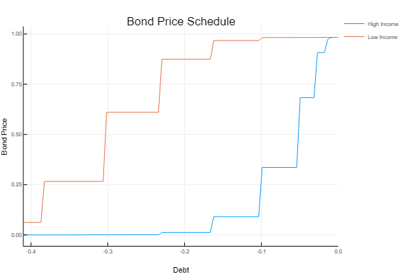
This code faithfully recreates Arellano’s Figure 3. We can see that it is more costly to borrow when bond holding are very low and approaches the risk free rate when bond holdings are high.

using Plots
tot = (1.0-vf.δpol)/(1.0 + vf.r)
plot(Bs[10:101], [tot[11,10:101], tot[14,10:101]], label = ["High" "Low"], xlabel = "B", ylabel = "q")

Recreating Arellano

Continuous Approximation

The discrete solution method paved over a few difficulties in solving this model. First, integrating the default probabilities was reduced to summing probabilities over a finite number of states. Similarly, finding the optimal level of bond holdings was reduced to checking all possible levels and selecting he maximum one, a process that is not feasible with continuous states. Finally, our value function will have a kink in it, meaning we will want to concentrate grid points around the kink for a better approximation. However, the location of the kink will change at each stage of the value function iteration, necessitating we either specify a fine grid or choose our grid endogenously. Adaptive sparse grids provide a solution to each of these problems. The adaptivity only places grids at points where our interpolation approximation is poor, meaning that they can approximate kinked functions closely without adding unnecessary points. The simple linear basis functions make integration and differentiation straightforward, so we can use the built in differentiation to employ a bisection search to find the optimal level of bond holdings and use the built in integration to calculate the default probabilities.

It should be noted that using continuous methods to solve this model is not merely an academic exercise. Martinez et. al. (2010) found that the results in Aguiar and Gopinath (2006) and Arellano (2008) could be sensitive to the discretization that they use. It is therefore important that researchers have methods of solving these models that don’t rely on discretization.

I have stored the adaptive sparse grid code used to solve this model here.

include("[filepath]/AdaptiveSparseGrid/fastasgd.jl")
using fastasgd
using FastGaussQuadrature

d = 2 # Number of Dimesions (2 because we are solving over income (y) and debt (B))
states = 1 # Number of discrete states (none)
ord = 11 # Maximum depth of approximation

# Bounds for B and y
lb = [-0.45, exp(ys)[1]]
ub = [0.45, exp(ys)[end]]

# Interpolation Objects
V_ = ASG(d, states, ord, lb, ub);
V_t = ASG(d, states, 18, lb, ub);
δ_ = ASG(d, states, ord, lb, ub);
Vd = ASG(1, states, ord, [lb[2]], [ub[2]]);
Vdt = ASG(1, states, ord, [lb[2]], [ub[2]]);
Vc = ASG(d, states, ord, lb, ub);
δt = ASG(1, 1, 14, [lb[2]-0.1], [ub[2]+0.1]);

# Initialize Values for Interpolation Objects
@time adaptivegrid( V_, x -> 0.0, 0.0001, 0.01, 1);
@time adaptivegrid( δ_, x -> 1.0, 0.0001, 0.01, 1);
@time adaptivegrid( Vd, x -> 0.0, 0.0001, 0.01, 1);
@time adaptivegrid( Vc, x -> 0.0, 0.0001, 0.01, 1);

We will frequently be evaluating expectations such as $\int V(B^{\prime}, y^{\prime}) dF(y, y^{\prime})$ . This expectation can be closely approximated using Gauss-Hermite quadrature. We therefore will use the FastGaussQuadrature package to calculate $4$ nodes for the approximation

# Gauss-Hermite for Apporximation Integral
nodes, weights = gausshermite(4);
weights = weights / sqrt(π);

To ensure type stability, I create another custom type to store all of the model parameters as well as the nodes and weights for quadrature.

type modelprimitives
    β::Float64
    σ::Float64
    r::Float64
    θ::Float64
    ŷ::Float64
    ρ::Float64
    η::Float64
    nodes::Array{Float64, 1}
    weights::Array{Float64, 1}
    
    function modelprimitives(β, σ, r, θ, ŷ, ρ, η, nodes, weights)
        return new(
            β, σ, r, θ, ŷ, ρ, η, nodes, weights
        )
    end
end
mp = modelprimitives(β, σ, r, θ, ŷ, ρ, η, nodes, weights);

Solving for Optimal Bond Holdings

The first step is to define the mapping for the value of default. This function is fairly simple as there is no optimum to solve for. We take the current guess for $V$ and $V_d$ , calculate utility in autarky and the expected value next period of autarky given our guess and use these values to update to $V_d$ . Again, we use quadrature to evaluate the expectation.

function TVd(y::Float64, V::ASG, Vd::ASG, mp::modelprimitives )
    expt = 0.0 
    for s = 1:length(mp.nodes)
        y′ = exp(sqrt(2.0)*mp.η*mp.nodes[s] + mp.ρ*log(y)) 
        expt += mp.weights[s] * (mp.θ * V(0.0, y′, 1) + (1.0 - mp.θ)*Vd(y′, 1) )  
    end
    
    return u( h( y, mp ), mp) + mp.β*expt
end

Next, we need to update the value function given that the government continues servicing its debt. To do this, we need a guess for the value function $V$ and the default probabilities $\delta$ . Using these guesses, we need to solve for the optimal amount of debt $B^{\prime}$ . Assuming that there is a single maximum in the range $[-0.45, 0.45]$ (a strong assumption but one that works here), the maximum of the value function will occur when $TV_c^{\prime}(B^{\ast}) = 0$ and if $TV_c^{\prime}(B) \textgreater 0$ , then $B \textless B^{\ast}$ . Similarly, if $TV_c^{\prime}(B) \textless 0$ then $B \textgreater B^{\ast}$ . We can then use a simple bisection method, where we start with $B_l = -0.45$ and $B_h = 0.45$ . Our candidate point becomes $B_t = \frac{B_l + B_h}{2}$ . If $TV_c^{\prime}(B_t) \textgreater 0$ , then we set $B_h = B_t$ . Otherwise we set $B_l = B_t$ . This process will eventually converge to the optimal value of $B^{\prime}$ . However, this requires us to know the derivative of our guesses $V$ and $\delta$ with respect to $B^{\prime}$ . Adaptive sparse grids make this easy to calculate, because they just require us to take the derivatives of the simpler basis functions. My program is set-up so that V(B′, y, 1) interpolates the function at the point (B′, y) and V(1, B′, y, 1) calculates the derivative with respect to the first argument.

This code is the derivative of the contraction operator with respect to $B^{\prime}$ .

function TVc′(y::Float64, B::Float64, B′::Float64, V::ASG, δ::ASG, mp::modelprimitives )
    expt = 0.0
    for s = 1:length(mp.nodes)
        y′ = exp(sqrt(2.0)*mp.η*mp.nodes[s] + mp.ρ*log(y)) 
        expt += mp.weights[s] *  V(1, B′, y′, 1) 
    end
    c =  y - (1.0 - δ(B′, y, 1))/(1.0 + mp.r)*B′ + B
    return max(c, 0.0)^(-mp.σ)*(-(1.0 - δ(B′, y, 1))/(1.0 + mp.r) + δ(1, B′, y, 1)/(1.0 + mp.r)*B′ ) + mp.β*expt    
    
end

Here is the bisection method to solve for the maximum.

function TVc(y::Float64, B::Float64, V::ASG, δ::ASG, mp::modelprimitives )
    B′L = V.lb[1]
    B′H = V.ub[1]-0.001
    eps = 1.0
    count = 0
    B′ = B′H
    f1 = 0.0
    while (eps > 1e-8)*(count = 0.0 )
        eps = abs(B′ - (B′L + B′H)/2.0)
        B′ = (B′L + B′H)/2.0

        f1 = TVc′(y, B, B′, V, δ, mp )

        if 0.0 <= f1
            B′L = B′
        elseif f1 < 0.0
            B′H = B′
        else
            break
        end
        count += 1
    end
    abs(B′ -  V.lb[1]) < 1e-3 && (B′ =  V.lb[1])
    expt = 0.0
# Using quadrature for the expectation
    for s = 1:length(mp.nodes)
        y′ = exp(sqrt(2.0)*mp.η*mp.nodes[s] + mp.ρ*log(y)) 
        expt += mp.weights[s] *  V(B′, y′, 1)
    end
    c = y - (1.0 - δ(B′, y, 1))/(1.0 + mp.r)*B′ + B

    return u( max(c, 0.0), mp) + mp.β*expt
end

Integrating the Default Probabilities

The default probabilities are merely the integral of the PDF for the income process over the default set. Note that in general the default set could be made up of disjoint subsets, so this integral is not trivial to approximate. To overcome this difficulty, I use adaptive sparse grids to approximate the PDF over the area where $V_c \textless V_d$ and set the function to zero otherwise. I then use the integrals of the simpler basis functions to approximate the integral of the true PDF. I do this process for a given point $B$ and $y$ , and for candidate value functions $V_c$ and $V_d$ .

function solδ(B::Float64, y::Float64, δt::ASG, Vc::ASG, Vd::ASG)
    adaptivegrid( δt, x -> ifelse(Vd(x[1], 1) > Vc(B, x[1], 1), 1.0/sqrt(2.0*pi*mp.η^2)*exp(-(log(x[1])-mp.ρ*log(y))^2/(2*mp.η^2))/x[1], 0.0), 0.0001, -0.00001, 1);
    u1 = deepcopy(δt.ub) 
    return min(iinterpolate(u1, δt, δt.l, 1), 1.0)
end

Value Function Iteration

We can combine the above pieces of code into a contraction. Here I only use 15 iterations, which gives a fairly close approximation. I am still working on a good metric for checking the convergence of a contraction with adaptive sparse grids. There are many approximations that give very close answers but have different points with non-zero hierarchical surpluses, making a comparison of the hierarchical surpluses a poor approximation of the contraction error. One possibility is using Gauss-Legendre quadrature to approximate the average error to the Euler Equation, but I have not found a great implementation yet. The code is not very fast, mainly because I use low pruning coefficients. The speed can be increased by loosening the pruning coefficients and using a more robust solver than the bisection method.

@time for i = 1:15
    adaptivegrid( Vc, x -> TVc(x[2], x[1], V_, δ_, mp), 0.01, 0.001, 1);
    adaptivegrid( Vd, x -> TVd(x[1], V_, Vdt, mp), 0.01, 0.001, 1);
    adaptivegrid( V_, x -> max(Vd(x[2],1), Vc(x[1], x[2], 1)), 0.001, 0.00001, 1);
    Vdt = deepcopy(Vd)
    adaptivegrid( δ_, x -> solδ(x[1], x[2], δt, Vc, Vd), 0.001, 0.00001, 1);
    @show Vc(-0.4, 1.0,1) - Vd(1.0,1)
end

262.525034 seconds (931.77 M allocations: 38.152 GB, 2.87% gc time)

The below figure compares the continuous solution with Arellano’s original solution, showing that they are very similar. We can see that the bond price increases with bond holdings. Remember that you must pay $1$ unit tomorrow to receive $q(B^{\prime}, y)$ units today. So for large negative holdings of debt, the cost of debt is quite high.

Continuous Vs Discrete 2

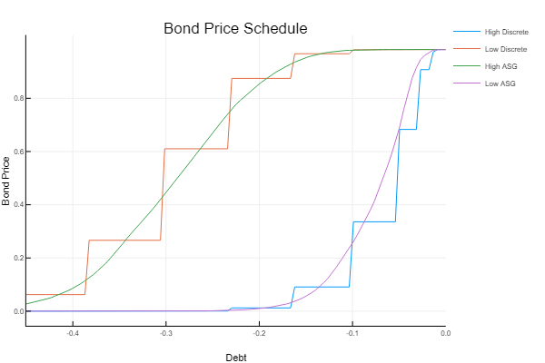
This figure recreates Arellano’s Figure 2, for the calibrated model. The default set is empty in the high state around $-0.1$ and in the low state around $-0.02$ . That means that the default risk set in the high state is effectively $[-0.23, -0.1]$ and in the low state is $[-0.05,-0.01]$ . These are the regions of risky contracts that occur in equilibrium.

Resources Available for Consumption 2

References

Arellano, Cristina. 2008. “Default Risk and Income Fluctuations in Emerging Economies.” American Economic Review, 98 (3): 690-712.
Hatchondo, Juan Carlos and Martinez, Leonardo and Sapriza, Horacio, Quantitative Properties of Sovereign Default Models: Solution Methods Matter (April 2010). IMF Working Papers, Vol. , pp. 1-28, 2010.
Tauchen, George, 1986. “Finite state markov-chain approximations to univariate and vector autoregressions,” Economics Letters, Elsevier, vol. 20(2), pages 177-181.

Model Overview

Discrete Approximation

Tauchen’s Method

Value Function Iteration

Continuous Approximation

Solving for Optimal Bond Holdings

Integrating the Default Probabilities

Value Function Iteration

References

Share this:

Like this:

Leave a Reply Cancel reply