Conditional Choice Probability and Nested Pseudo-Likelihood Estimators

The Nested Fixed Point algorithm proposed by John Rust is a generally applicable model that is easy to extend. However, it tends to be computationally burdensome because it requires an optimizer to solve for the value function for each parameter guess. In their paper “Conditional Choice Probabilities and the Estimation of Dynamic Models” Hotz and Miller show that under the assumptions made by Rust using a contraction mapping to solve for the value function is unnecessary. They provide a simple inversion which yields similar estimates to the Nested Fixed Point algorithm in a fraction of the run time. Aguirregabiria and Mira extended the idea of Hotz and Miller to derive an estimator, the Nested Pseudo-Likelihood estimator, that is asymptotically equivalent to the Nested Fixed Point algorithm and has similar computational gains to the Conditional Choice Probability estimator (see “Swapping the Nested Fixed Point Algorithm: A Class of Estimators for Discrete Markov Decision Models”). The description and code is based on Rust (1987), Hotz and Miller (1993), and Aguirregabiria and Mira (2002) as well as their online supplementary material. The data is the bus engine replacement data used in Rust’s original paper, and that I use in my description of the Nested Fixed Point algorithm (see here). You can run the code on that page to generate the input dataset.

Remember that the agent’s problem is characterized by the Bellman equation

$V(x) = \int \max_d \left\{ u(x,d) + \epsilon(d) + \beta \sum_{x^{\prime}}V(x^{\prime})p(x^{\prime}\vert x, d)\right\}g(d\epsilon \vert x)$

which can be rewritten as

$V(x) = \sum_{d}P(d \vert x) \left(u(x,d) + \frac{1}{P(d \vert x)}\int \epsilon(d) I\left\{ d \in \text{argmax} \left[v(x,d) + \epsilon(d) \right] \right\}g(d\epsilon \vert x) + \beta \sum_{x^{\prime}}V(x^{\prime})p(x^{\prime}\vert x, d) \right)$

where

$P(d \vert x) = \int I\left\{ d \in \text{argmax} \left[v(x,d) + \epsilon(d) \right] \right\}g(d\epsilon \vert x)$

The key insight that Hotz and Miller made was that we can solve this equation for $V(x)$ in terms of the other expressions. Consider our discrete case in matrix notation. Then

$\left[ \begin{matrix} V(0) \\ V(1)\\ V(2)\\ \vdots\\ V(n) \\ \end{matrix} \right] = \sum_d \left[ \begin{matrix} P(0, d) \\ P(1, d)\\ P(2, d)\\ \vdots\\ P(n, d) \\ \end{matrix} \right] * \left( \left[ \begin{matrix} u(0, d) \\ u(1, d)\\ u(2, d)\\ \vdots\\ u(n, d) \\ \end{matrix} \right]+ \left[ \begin{matrix} e(0, d, P) \\ e(1, d, P)\\ e(2, d, P)\\ \vdots\\ e(n, d, P) \\ \end{matrix} \right] + \left[ \begin{matrix} \pi_0 & \pi_1 & \pi_2 & 0 & 0 & \cdots & 0 & 0\\ 0 & \pi_0 & \pi_1 & \pi_2 & 0 & \cdots & 0 & 0\\ 0 & 0 & \pi_0 & \pi_1 & \pi_2 & \cdots & 0 & 0\\ \vdots & & & & \ddots & & & \vdots\\ 0 & 0 & 0 & 0 & 0 & \cdots & 0 & 1 \\ \end{matrix} \right] \left[ \begin{matrix} V(0) \\ V(1)\\ V(2)\\ \vdots\\ V(n) \\ \end{matrix} \right] \right)$

where $*$ denotes row-wise multiplication, rather than standard matrix multiplication and

$e(x, d, P) = \frac{1}{P(d \vert x)}\int \epsilon(d) I\left\{ d \in \text{argmax} \left[v(x,d) + \epsilon(d) \right] \right\}g(d\epsilon \vert x)$

In the notation of Aguirregabiria and Mira, we can write this more compactly as

$V = \sum_{d} P(d) * \left[ u(d) + e(d,P) + \beta F(d)V\right]$

Rearranging the terms shows that

$V = \left(I - \beta \sum_{d} P(d) * F(d) \right)^{-1}\sum_{d} P(d) * \left[ u(d) + e(d,P)\right]$

When estimating a Rust model we compute nonparameteric estimates of $F(d)$ , i.e. the state transition probabilities. Notice that we can estimate the choice probabilities $P(d \vert x)$ nonparameterically as well. With an explicit functional form for $u$ and for the errors $\epsilon$ we are able to compute the term $u(d) + e(d,P)$ as well, meaning that we can estimate $V$ without using a contraction mapping. Estimating the parameters of the model depends on $u$ and $e$ , so for the rest of this discussion I will use the linear case in Rust’s original paper, i.e.

$u(0, x) = -\theta_{11} x$

and

$u(1, x) = - RC$

and assume errors are distributed Type I extreme value. The assumption of Type I extreme value errors actually provides a closed form solution for $e(d, P)$ . Note that

$E\left[\max_d \{v(x,d) + \epsilon(d)\}\ \vert\ x\right] = \gamma + \ln \sum_d e^{v(x,d)}$

This comes from the fact that the maximum of Type I extreme value random variables is again a Type I extreme value random variable and these all have expectation $\gamma \sigma + \alpha$ (where $\sigma$ is the standard deviation and $\alpha$ is the location parameter). Note that we can rewrite

$E\left[\epsilon\ \vert\ d \in \text{argmax} \left[v(x,d) + \epsilon(d) \right] \right] = E\left[ \max_j \{v(x,j) + \epsilon(j) \} - v(x,d) \right]$

and, after pulling the nonstochastic $v(x,d)$ out of the expectation, this becomes

$E\left[\epsilon\ \vert\ d \in \text{argmax} \left[v(x,d) + \epsilon(d) \right] \right] = \gamma + \ln \sum_j e^{v(x,j)} - v(x,d) = \gamma - \ln P(d\ \vert\ x)$

We therefore have the two expressions for $u(d) + e(d,P)$
1. $d = 0$ and $u(0) + e(0,P) = -\theta_{11} x + \gamma \ln P(0\ \vert\ x)$
2. $d = 1$ and $u(1) + e(1,P) = -RC + \gamma \ln P(1\ \vert\ x)$

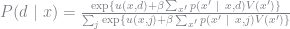
Remember that $P(d\ \vert\ x)$ is estimated nonparametrically and we are interested in estimating the parameters $\theta = (RC, \theta_{11})$ . The two most common ways of estimating these parameters is through GMM and Maximum Likelihood. The key to both is to recover the choice probabilities from an estimate of $V$ given some parameter guess $\theta_0$ . Note that $V$ can be written as

$V(x) = \gamma + \ln \sum_d \exp\{u(x,d) + \beta \sum_{x^{\prime}} p(x^{\prime}\ \vert\ x, d)V(x^{\prime})\}$

A theorem by Williams, Daly, and Zachary says that the choice probabilities are equal to

$P(d\ \vert\ x) = \frac{\partial V(x)}{\partial v(x,d)}$

where again, $v(x,d) =u(x,d) + \beta \sum_{x^{\prime}} p(x^{\prime}\ \vert\ x, d)V(x^{\prime})$ . Under our assumptions equals

$P(d\ \vert\ x) = \frac{\exp\{u(x,d) + \beta \sum_{x^{\prime}} p(x^{\prime}\ \vert\ x, d)V(x^{\prime})\}}{\sum_{j} \exp\{u(x,j) + \beta \sum_{x^{\prime}} p(x^{\prime}\ \vert\ x, j)V(x^{\prime})\}}$

In the case of GMM we wish to find the parameters $\theta$ such that the moment condition $E[d_i - P(d_i\ \vert x_i, \theta)\ \vert\ x_i] = 0$ holds, i.e. the predicted probabilities match the empirical probabilities. We can do this by finding a set of instruments $Z_i$ and create sample moments

$g_n(\theta) = \sum_i z_i^{\prime}\left(d_i - P(d_i\ \vert x_i, \theta) \right)$

and find the parameter values that minimize $g_n(\theta)^{\prime}g_n(\theta)$ . Because $x_i$ is assumed exogenous it can act as an instrument for itself. I also use a constant as an instrument. This amounts to requiring the estimated choice probabilities and expected value of $x_i$ equal their empricial counterparts. For Maximum Likelihood we want to find the parameters that maximize the the log likelihood function

$LL(\theta) = \sum_i \left( d_i \ln P(d_i\ \vert\ x_i, \theta) + (1-d_i) \ln P(1 -d_i\ \vert\ x_i, \theta) \right)$

Non-parametric Transition Probabilities

This calculation is the same that was done in Rust’s original paper. The state space is discretized and each transition probability is estimated with a simple frequency estimator.

pi_1 = sum( [x == 0 for x in inputDataset[3] ] )/length(inputDataset[3])
pi_2 = sum( [x == 1 for x in inputDataset[3] ] )/length(inputDataset[3])
pi_3 = 1 - pi_1 - pi_2

function transition_probs(trans)
    t = length(trans)
    ttmp = zeros(K - t, K) # Transition Probabilities
    for i in 1:K - t
        for j in 0:t-1
            ttmp[i, i + j] = trans[j+1]
        end
    end
    atmp = zeros(t,t) # Absorbing State Probabilities
    for i in 0:t - 1
        atmp[i+ 1,:] = [zeros(1,i) trans[1:t - i - 1]' ( 1 - sum(trans[1:t- i - 1]) ) ]
    end
    return [ttmp ; zeros(t, K - t) atmp]
end;
transition_probs( [pi_1, pi_2, pi_3])

Non-parametric or Kernel Based Choice Probabilities

If the data is sufficiently rich enough, we can use a simple frequency estimator to get our estimated choice probabilities. The problem with this is that for many states the estimated probability will likely be $0$ . This would imply that our value function is equal to $-\infty$ in these states (because we need to take the log of $0$ ) and leads to problems in estimation.

uniqX = unique(inputDataset[:dtx])
baseMat = convert(Matrix, inputDataset)
nonpar = zeros( uniqX )

count = 1
for i in uniqX
    sub = baseMat[inputDataset[:dtx] .== i, :]
    nonpar[count] = sum(sub[:,1])/size(sub,1)
    count += 1
end
nonpar

78-element DataArrays.DataArray{Float64,1}:
 0.0      
 0.0      
 0.0      
 0.0      
 0.0      
 0.0      
 0.0      
 0.0      
 0.0      
 0.0      
 0.0      
 0.0      
 0.0      
 ⋮        
 0.0714286
 0.0      
 0.0      
 0.0      
 0.125    
 0.0      
 0.25     
 0.0      
 0.0      
 0.0      
 0.0      
 0.5

An alternative is to estimate the choice probabilities by using a smooth probability function. Here I use a standard logit regression, where my right-hand side consists of power of the state variable. This should allow us to match the empirical probabilities fairly well

using GLM, DataFrames

inputDataset[:dtx2] = inputDataset[:dtx].^2
inputDataset[:dtx3] = inputDataset[:dtx].^3
model = glm(@formula(dtc ~ dtx + dtx2 + dtx3), inputDataset, Binomial(), LogitLink())

DataFrames.DataFrameRegressionModel{GLM.GeneralizedLinearModel{GLM.GlmResp{Array{Float64,1},Distributions.Binomial{Float64},GLM.LogitLink},GLM.DensePredChol{Float64,Base.LinAlg.Cholesky{Float64,Array{Float64,2}}}},Array{Float64,2}}

Formula: dtc ~ 1 + dtx + dtx2 + dtx3

Coefficients:
               Estimate  Std.Error  z value Pr(>|z|)
(Intercept)     -18.553    4.39745 -4.21904    <1e-4
dtx            0.833554   0.295884  2.81717   0.0048
dtx2         -0.0156818 0.00638369 -2.45654   0.0140
dtx3         9.92305e-5 4.40502e-5  2.25267   0.0243

x = 1:1:K
tmp = -hcat(ones(x), x, x.^2, x.^3) *coef(model)
prob0 = 1./(1 + exp(tmp))
prob0 = hcat(1-prob0, prob0);

Estimating the Value Function

Using our estimates of the choice probabilities and the state transition probabilities, our estimate of $V$ will be given by

$\hat{V} = \left(I - \beta \sum_{d} \hat{P}(d) * \hat{F}(d) \right)^{-1}\sum_{d} \hat{P}(d) * \left[ u(d) + e(d,\hat{P})\right]$

Of course, this requires that $u(d)$ is known. Note however, that if utility is linear in parameters, i.e. $u(d,\theta) = h(d)^{\prime}\theta$ , then we can define $V$ in terms of $\theta$ as follows

$\hat{V}(\theta) = \left(I - \beta \sum_{d} \hat{P}(d) * \hat{F}(d) \right)^{-1}\sum_{d} \hat{P}(d) * \left[ h(d)^{\prime}\theta + e(d,\hat{P})\right]$

where the term $\sum_{d} \hat{P}(d) * h(d)^{\prime}$ is computeable from the data. We therefore need to calculate the following terms

$H_1(d) = \left(I - \beta \sum_{d} \hat{P}(d) * \hat{F}(d) \right)^{-1}\sum_{d} \hat{P}(d) * h(d)^{\prime}$

and

$E_1(d) = \left(I - \beta \sum_{d} \hat{P}(d) * \hat{F}(d) \right)^{-1}\sum_{d} \hat{P}(d) * e(d,\hat{P})$

so that

$\hat{V}(\theta) = H_1 \theta + E_1$

The choice probabilities will then be based on the terms

$\tilde{P}(d) = \frac{\exp\left(h(d)^{\prime}\theta + \beta \hat{F}(d) H_1(d) \theta + \beta \hat{F}(d) E_1(d)\right)}{\sum_j \exp\left(h(j)^{\prime}\theta + \beta \hat{F}(j) H_1(j) \theta + \beta \hat{F}(j) E_1(j)\right)}$

or combining $h(d)^{\prime}\theta$ and $\beta \hat{F}(d) H_1(d)$

$\tilde{P}(d) = \frac{\exp\left( \left[h(d)^{\prime} + \beta \hat{F}(d) H_1(d) \right] \theta + \beta \hat{F}(d) E_1(d)\right)}{\sum_j \exp\left( \left[h(j)^{\prime} + \beta \hat{F}(j) H_1(j) \theta \right] + \beta \hat{F}(j) E_1(j)\right)}$

baseTrans = [transition_probs( [pi_1, pi_2, pi_3]), ones(K, 1) .* hcat( [pi_1 pi_2 pi_3], zeros(1, K-3))]
baseData = convert(Matrix, inputDataset);
y = baseData[:,1];

h_base = [ hcat( zeros(K,1), (1:1:K) .* -0.001 ), hcat(-ones(K, 1), zeros(K,1)) ]

F_hat = sum([prob0[:,i].*baseTrans[i] for i = 1:size(prob0,2)])
H_hat = sum([prob0[:,i].*h_base[i] for i = 1:size(prob0,2)])
E_hat = sum( [prob0[:,i].*(eulergamma - log( prob0[:,i] ) ) for i = 1:size(prob0,2)])
I_F = eye(90) - beta * F_hat

H1 = (inv(I_F)*H_hat)
E1 = (inv(I_F)*E_hat)

H_d = [h_base[i] + beta * baseTrans[i] * H1 for i = 1:size(prob0,2)]
E_d = [beta * baseTrans[i] * E1 for i = 1:size(prob0,2)];

nalt = convert(Int, maximum(y+1) );
npar = convert(Int, size(zobs,2)/nalt )

function choice_p( theta ) # Computes the choice probabilities for a given parameter estimate
    choiceP = zeros(90,2) ;

    for d = 1:npar
        choiceP[:,d] = H_d[d] * (theta  ) + E_d[d] ;
    end

    choiceP = choiceP .- maximum(choiceP, 2)  ; # Correct for Overflow
    choiceP = exp(choiceP)./sum(exp(choiceP), 2) ;
    return choiceP
end
example = choice_p([9.26, 0.5])

90×2 Array{Float64,2}:
 0.999905  9.51939e-5 
 0.999894  0.000106292
 0.999881  0.000118597
 0.999868  0.000132228
 0.999853  0.000147318
 0.999836  0.000164008
 0.999818  0.000182456
 0.999797  0.000202829
 0.999775  0.000225314
 0.99975   0.00025011 
 0.999723  0.000277437
 0.999692  0.000307533
 0.999659  0.000340659
 ⋮                    
 0.909938  0.0900616  
 0.895735  0.104265   
 0.878673  0.121327   
 0.858287  0.141713   
 0.834192  0.165808   
 0.806229  0.193771   
 0.774621  0.225379   
 0.740131  0.259869   
 0.704121  0.295879   
 0.66855   0.33145    
 0.636857  0.363143   
 0.626109  0.373891

x_state = convert(Array{Int64}, baseData[:,2])
hobs = [H_d[i][x_state, :] for i = 1:npar]
eobs = [E_d[i][x_state, :] for i = 1:npar];

GMM Estimator

As mentioned earlier, we can use a simple GMM estimator to generate $\hat{\theta}$ . I choose $z_i = (1, x_i)$ as my set of instruments and minimize a quadratic form in.

$g_n(\theta) = \sum_i z_i^{\prime}\left(d_i - P(d_i\ \vert x_i, \theta) \right)$

I use the identity matrix as my GMM weighting matrix, so that the estimator ultimately minimizes $g_n(\theta)^{\prime}g_n(\theta)$ . It would be easy enough to find the derivatives of this objective function with respect to the parameters and use a gradient based optimizer. However, because the dataset is so small I use a gradient-free search instead.

x = baseData[:,2]

using Optim

function gmm( x, y )

    function objFunc( params )
        p_1 = choice_p(params)[convert(Array{Int},x),:]
        firstX = [ones(x) x][convert(Array{Int64},y) .== 1,:]
        g1 = sum(firstX,1)'/size(p_1,1) .- [ mean(p_1[:,2],1) x'p_1[:,2]/size(x,1)]'
        moment = (g1'g1)[1]

        return moment
    end

    params0 = [9, 2.5]
    optimum = optimize( objFunc, params0, Optim.Options(g_tol = .00000001, iterations = 200) )
    return optimum
end

@time ot = gmm(x,y)

0.299201 seconds (174.64 k allocations: 33.829 MB, 2.71% gc time)

Results of Optimization Algorithm
 * Algorithm: Nelder-Mead
 * Starting Point: [9.0,2.5]
 * Minimizer: [9.741156194406098,2.3781350832783184]
 * Minimum: 1.015810e-07
 * Iterations: 24
 * Convergence: true
   *  √(Σ(yᵢ-ȳ)²)/n < 1.0e-08: true
   * Reached Maximum Number of Iterations: false
 * Objective Function Calls: 29

The parameter estimates are very close the the $2.62749$ and $9.75822$ that Rust estimates using the Nested Fixed Point Algorithm. Using a gradient-free search with the Nested Fixed Point Algorithm found the parameter estimates in $199$ seconds whereas the GMM estimator found them in $0.299$ seconds, so there is a considerable savings in run time.

(Pseudo) Maximum Likelihood Estimator

The maximum likelihood estimator is given by the $\hat{\theta}$ that maximizes the following expression (or equivalently minimizes its negative)

$LL(\theta) = \sum_i \left( d_i \ln P(d_i\ \vert\ x_i, \theta) + (1-d_i) \ln P(1 -d_i\ \vert\ x_i, \theta) \right)$

We don’t know the true choice probabilities as we aren’t actually evaluating them at the true parameter values, thus the “pseudo” in the name. Again, you could use a more efficient algorithm such as BHHH to estimate the coefficients but a simple gradient-free search finds the maximum quickly given the size of the data. As we increase the number of parameters we are estimating and the size of the action/state space it becomes more important to program efficient estimation routines.

function mle( x, y )

    function ll( params )
        ll = 0
        phat = choice_p( params )[convert(Array{Int}, x), :]
        for d = 1:npar

            ll = ll + sum( (y + 1 .== d) .* log( phat[:,d] .* ( phat[:,d].>=1e-16) + ( phat[:,d].<1e-16)*1e-16 ), 1 )
        end

        return -ll[1]
    end

    params0 = [9, 2.5]
    optimum = optimize( ll, params0, Optim.Options(g_tol = .000000001, iterations = 200) )
    return optimum
end

@time mle(x,y)

0.180965 seconds (103.55 k allocations: 125.531 MB, 7.56% gc time)

Results of Optimization Algorithm
 * Algorithm: Nelder-Mead
 * Starting Point: [9.0,2.5]
 * Minimizer: [9.615647287663599,2.4341254946997073]
 * Minimum: 3.007268e+02
 * Iterations: 43
 * Convergence: true
   *  √(Σ(yᵢ-ȳ)²)/n < 1.0e-09: true
   * Reached Maximum Number of Iterations: false
 * Objective Function Calls: 49

The parameter estimates are again very close the the $2.62749$ and $9.75822$ that Rust estimates using the Nested Fixed Point Algorithm with comparable savings in run time.

Nested Pseudo-Likelihood Estimator

One might wonder if there is any advantage to using Maximum Likelihood or GMM for estimation. Somewhat surprisingly there is. Astute readers will notice that we started off with an initial estimate of the choice probabilities, $\hat{P}(d\ \vert\ x)$ , and end the estimation routine with a different set of estimates for the choice probabilities, $\tilde{P}(d\ \vert\ x)$ . This means that our value function is approximated with a different set of choice probabilities than we end up with, which seems inconsistent. Ultimately, we could repeat our estimation procedure many times, each time using the new choice probabilities. Aguirregabiria and Mira show that when using pseudo maximum likelihood estimates this process is actually a contraction, and that it is equivalent to Rust’s Nested Fixed Point algorithm. For a full discussion, see their paper “Swapping the Nested Fixed Point Algorithm: A Class of Estimators for Discrete Markov Decision Models”. Below is a brute force implementation of their NPL estimator using the previously written code. As you can see, the parameter estimates are identical to Rust’s (up to a few decimal places because I use different tolerances) but are computed in a fraction of the time.

tmpP= choice_p([9.26, 0.5])
function npl( x,y )
    param = [9, 2.5]
    prob0 = tmpP
    criterion = 1e-6
    criter = 1
    optimum = []
    function choice_p( theta, H_d, E_d ) # Computes the choice probabilities for a given parameter estimate
        choiceP = zeros(90,2) ;

        for d = 1:npar
            choiceP[:,d] = H_d[d] * theta + E_d[d] ;
        end

        choiceP = choiceP .- maximum(choiceP, 2)  ; # Correct for Overflow
        choiceP = exp(choiceP)./sum(exp(choiceP), 2) ;
        return choiceP
    end

    while criter > criterion
        F_hat = sum([prob0[:,i].*baseTrans[i] for i = 1:size(prob0,2)])
        H_hat = sum([prob0[:,i].*h_base[i] for i = 1:size(prob0,2)])
        E_hat = sum( [prob0[:,i].*(eulergamma - log( prob0[:,i] ) ) for i = 1:size(prob0,2)])
        I_F = eye(90) - beta * F_hat

        H1 = (inv(I_F)*H_hat)
        E1 = (inv(I_F)*E_hat)

        H_d = [h_base[i] + beta * baseTrans[i] * H1 for i = 1:size(prob0,2)]
        E_d = [beta * baseTrans[i] * E1 for i = 1:size(prob0,2)];

        function ll( params )
            ll = 0
            phat = choice_p( params, H_d, E_d  )[convert(Array{Int}, x), :]
            for d = 1:npar

                ll = ll + sum( (y + 1 .== d) .* log( phat[:,d] .* ( phat[:,d].>=1e-16) + ( phat[:,d].<1e-16)*1e-16 ), 1 )
            end

            return -ll[1]
        end

        optimum = optimize( ll, param, Optim.Options(g_tol = .00000000001, iterations = 200) )
        criter = maximum(abs(param - optimum.minimizer))
        param = optimum.minimizer
        prob0 = choice_p( param, H_d, E_d )

    end

    return optimum
end

@time npl(x,y)

4.435695 seconds (543.87 k allocations: 1.731 GB, 8.43% gc time)

Results of Optimization Algorithm
 * Algorithm: Nelder-Mead
 * Starting Point: [9.758346242453971,2.6276132009985553]
 * Minimizer: [9.758346242453971,2.6276132009985553]
 * Minimum: 3.002502e+02
 * Iterations: 46
 * Convergence: true
   *  √(Σ(yᵢ-ȳ)²)/n < 1.0e-11: true
   * Reached Maximum Number of Iterations: false
 * Objective Function Calls: 50

Non-parametric Transition Probabilities

Non-parametric or Kernel Based Choice Probabilities

Estimating the Value Function

GMM Estimator

(Pseudo) Maximum Likelihood Estimator

Nested Pseudo-Likelihood Estimator

Share this:

Like this:

Leave a Reply Cancel reply