Adaptive Sparse Grids

UPDATE: For an application of adaptive sparse grid code to a macro model, see here.

A major issue with macroeconomic models, and Bellman iteration in general, is the curse of dimensionality. We generally do not have a parametric form for the value function and so we must approximate its true value on some set of grid points and then interpolate for values off the grid. The problem is that the number of grid points increase exponentially with the dimension of the problem, i.e. . Sparse grids, to an extent, mitigate this issue. They rely on the observation that certain points are more important in the interpolation of a function. I follow the exposition given in Brumm and Scheidegger. My code for the multi-dimensional adaptive sparse grid is based off of the sparse grid interpolation algorithm Spinterp by Klimke and Wohlmuth. I have updated their algorithm to make the grid selection adaptive. This will be made clearer below.

using Plots

Collection of Basis Functions

All interpolation uses a collection of basis functions and weights to approximate a given function.

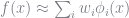
In the standard sparse grid literature, our basis functions are given by the hat function.

function φ(x)
    -1.0 <= x <= 1.0 && return 1 - abs(x)
    return 0.0
end

baseX = linspace(-1.0, 1.0, 500)
y = [φ(j) for j in baseX ]
plot(baseX , y, label = "Basis Function" )

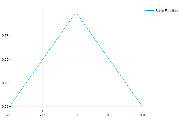
The original interval is then broken into subintervals, half of the original width, and the basis function is scaled to this new subinterval. So for level the new intervals are to and $latex  \frac{1}{2}$ to . The basis functions look as follows

# Collection of Basis Functions
s = 2 # Current step level
h = 2.0^(-s) # Grid size
x = linspace(0.0, 1.0, 400)
y = [[φ( (j - i*h)/h ) for j in x] for i = 1:2:2^s-1] # Note that the i's are all odd
plot(x, y, label = ["Basis Function 2,1" "Basis Function 2,3"])

Sparse Grid Interpolation

In order to demonstrate the technique it helps to look at the sample function used in Brumm/Scheidegger. The two things that you should note are that the function is smooth and that it disappears on the boundaries of the interval. The smoothness implies that the sparse grid is in a certain sense optimal. Because it disappears on the boundaries we can use a very simple sparse grid scheme. This scheme will need to be updated to the “Clenshaw-Curtis” scheme when we have nonzero values on the boundaries.

f = x -> x^2*sin(π*x)
yFunc = [f(j) for j in x]
plot(x, yFunc, label = "f")

The first approximation is simply the hat function, and we weight it by functions value at . This is not a very precise approximation as we can see below.

s = 1
h = 2.0^(-s)
x_i = [i*h for i = 1:2:2^s-1]
α_i = [f(x_ij) - (f(x_ij - h) + f(x_ij + h))/2 for x_ij in x_i]
y_1 = sum([[φ( (j - x_ij)/h )*α_ij for j in x] for (x_ij, α_ij) in zip(x_i, α_i)])
plot(x, [y_1 yFunc], label = ["Approximation" "Function"])

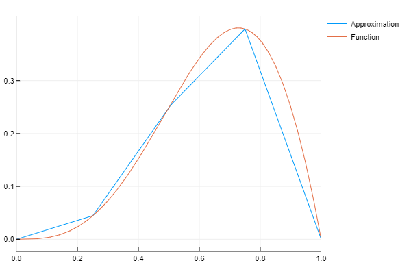
At the next level, we correct our approximation at two points, namely and . We want the approximation to be exact at three points now. Note that both of our new basis functions are at , so we do not need to change our original weight (this is one of the advantages of sparse grid interpolation, all previously calculated weights stay fixed as we move to more precise estimates). Our first approximation estimated the value at to be

Using this, we can see that a weight of will make our second degree approximation exact at . We can do a similar exercise for the point .

s = 2
h = 2.0^(-s)
x_i = [i*h for i = 1:2:2^s-1]

α_i = [f(x_ij) - (f(x_ij - h) + f(x_ij + h))/2 for x_ij in x_i]
y_2 = sum([[φ( (j - x_ij)/h )*α_ij for j in x] for (x_ij, α_ij) in zip(x_i, α_i)])
y_approx = y_1 .+ y_2

plot(x,[y_approx yFunc], label = ["Approximation" "Function"])

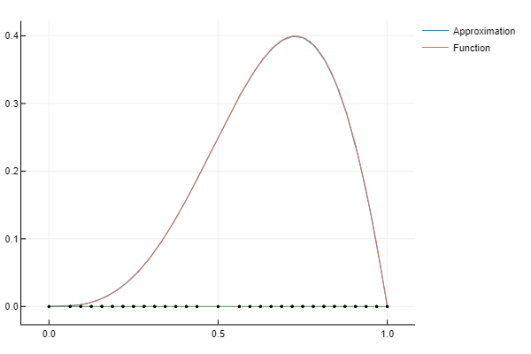
The previous step can be generalized. At each degree we can simple average the values of at the points and and subtract this value from to get our new weights. Then, adding together the approximation from all previous degrees will give our new approximation.

s = 3
h = 2.0^(-s)
x_i = [i*h for i = 1:2:2^s-1]

α_i = [f(x_ij) - (f(x_ij - h) + f(x_ij + h))/2 for x_ij in x_i]
y_3 = sum([[φ( (j - x_ij)/h )*α_ij for j in x] for (x_ij, α_ij) in zip(x_i, α_i)])
y_approx = y_1 .+ y_2 .+ y_3

plot(x,[y_approx yFunc], label = ["Approximation" "Function"])

This is already a fairly close approximation to a nonlinear function. Note that I have written out each iteration rather than put it into a formula to help elucidate the code, but we need to make this more compact to be practical.

Adaptive Sparse Grid

When it comes to interpolating a function, not all points are created equal. In the case of a linear function, only two points would be needed to “approximate” the function on an interval. So while we could sample 100 points and interpolate between them to “approximate” our linear function, 98 of those points would be a wasted calculation. Adaptive sparse grids apply this same logic to our approximating functions. Each points contribution to the approximation is proportional to its weight. So points with larger weights are more important.

function chld(value::Float64, level::Int )
    h = 2.0^(-level-1)
    return [value - h, value + h]
end

function AdptGrid1D( tol::Float64, f::Function )
    lst = Tuple[(0.5, f(0.5), 1, chld(0.5, 1))]
    ln0 = length(lst)
    ln1 = ln0 + 1
    i = 1
    @time while ln1 > ln0
        ln0 = ln1
        l = lst[i]
        for c in l[4]
            h = 2.0^(-l[3]-1)
            α_i = f(c) - (f(c - h) + f(c + h))/2
            abs(α_i) <= tol && push!( lst, (c, α_i, l[3]+1, chld(c, l[3]+1)) )
        end
        ln1 = length(lst)
        i += 1
    end
    push!(lst, (1.0, f(1.0), 1, []), (0.0, f(0.0), 1, []));
    return lst
end

Multi-dimensional Adaptive Sparse Grid

Part of the problems with the previous example is that the function was well approximated by an uniformly spaced grid. To demonstrate the computational costs that an adaptive grid can afford we will look at a two-dimensional function

Note that this function is also highly nonlinear, not possessing a derivative along the curver . Because the sparse grid approximation works best for smooth function so approximating this function posses a challenge.

Two-Dimensional Adaptive Sparse Grid Using Spinterp

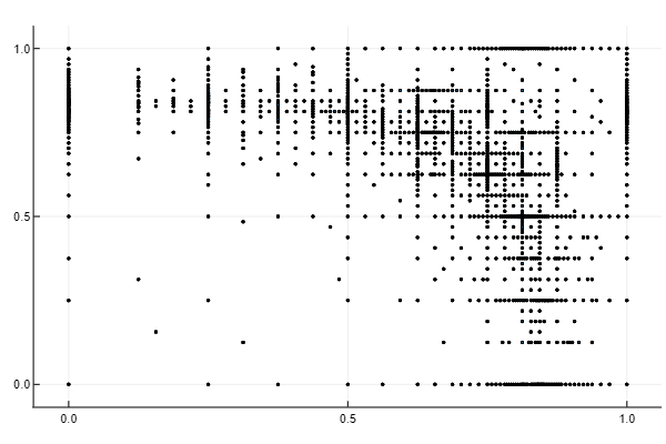
Klimke and Wohlmuth provide an algorithm for sparse grid interpolation called spinterp. Their formulation does not choose grid points in an adaptive manner so I had to change the basic algorithm to implement that feature. Additionally, their algorithm is defined for the region which is restrictive for most macroeconomic models. In anticipation of taking this to the standard growth model I have adapted their algorithm to work in a generic rectangular region. The code is not for the faint of heart, so I have included at the bottom of the page after the results. While I do not give an in-depth discussion of the algorithm, anyone interested can read the paper by Klimke and Wohlmuth. I found that it explains this complex procedure very well.

The below figure shows the points of evaluation for our interpolation. Note that the points cluster along the ridge where the derivative is not defined. In smooth areas, such as the lower left quadrant, only a few points are used to approximate the function.

box = [0.0 1.0; 0.0 1.0] # Define region of interpolation
b = box[:,2] # Get upper bounds
a = box[:,1] # Get lower bounds
nobs = 100 # Choose number of observations to interpolate, 100^2 = 10,000
x = linspace(a[1], b[1], nobs) # Create mesh for x axis
y = linspace(a[2], b[2], nobs) # Create mesh for y axis
f = (x,y) -> 1/(abs(0.5 - x^4 - y^4) + 0.1) # Define function to interpolate
d = 2 # Define dimension of the problem
n = 15 # Define the degree of the sparse grid algorithm

@time Znd, ΔHnd = spvals(f, d, n, b, a, .01); # Generate weights and nodes for ϵ >= 0.01

# Plot nodes
initPtsx = [x[1] for x in vcat(vcat(ΔHnd...)...)]
initPtsy = [x[2] for x in vcat(vcat(ΔHnd...)...)]
scatter(initPtsx, initPtsy, labels = "", marker = 1)

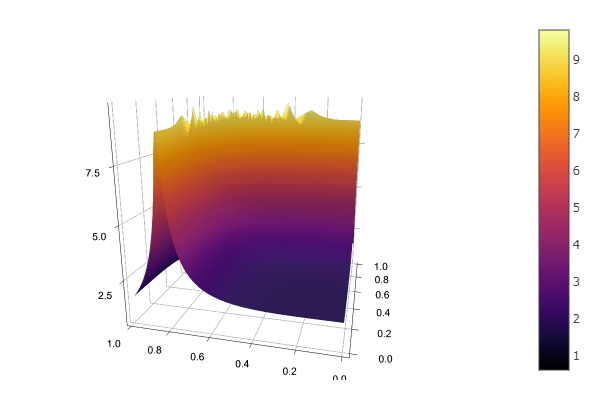
Below is a plot of the approximation using and . You can see that the ridge is roughly approximated but the rest of the function appears very smooth. This approximation was done with 2,339 points.

nd = 15-d # Maximum dimension of the interpolation
interVals = spinterp(d, nd, Znd, vcat(Base.product((x-a[1])/(b[1]-a[1]),(y-a[2])/(b[2]-a[2]))...), ΔHnd, b, a )
# Note that x and y are transformed to be in the unit interval before interpolating

@time z = reshape(interVals, nobs, nobs)'

#using Plots
Plots.surface(x,y,z, aspect_ratio=:equal)

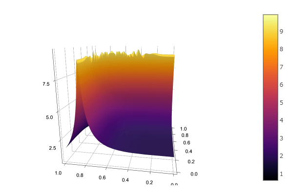
The adaptive sparse grid approximation might seem poor, so it is worth comparing to other methods of interpolation. First, consider a regular sparse grid of degree . This requires points to be evaluated and gives a considerably worse approximation.

Next consider bilinear interpolation. I used a grid size of and of to have a comparable calculation to the sparse grid approximations. The  grid performs much better than the regular sparse grid (which is unsurprising given that sparse grids are only optimal for smooth functions) but worse than the adaptive sparse grid. The  grid is comparable to the adaptive sparse grid but at the cost of more function evaluations. This highlights an important trade-off inherent in calculating sparse grids. We incur a higher computational cost in calculating the grid points and the interpolated values while having a lower computational cost in function evaluations. In this example, the trade-off is not in favor of the adaptive sparse grid. It took my computer seconds to calculate the adaptive grid and plot the interpolated values for this function, while it took my computer less than a fifth of a second to calculate a bilinear interpolation of the same function (which is considerably more precise). However, in most macro models, it will be the function evaluations that are costly as you need to perform some form of optimization at every grid point. In these cases, adaptive sparse grids tend to outperform bilinear interpolation.

Finally, here is a Chebyshev Polynomial interpolation, using points in each dimension and fitting with a polynomial of degree . As expected, the polynomial interpolation performs poorly as the function is not smooth.

Adaptive Sparse Grid Julia Code

The code that I used for the above figures can be found here.

UPDATE: I have written some more efficient adaptive sparse grid code which can be found here.

References

• Brumm, J., Scheidegger, S. (2017). “Using Adaptive Sparse Grids to Solve High-Dimensional Dynamic Models”. (Econometrica, Vol. 85, No. 5 (September, 2017), 1575–1612)
• Klimke, A., Wohlmuth, B. (2005). “Algorithm 847: Spinterp: piecewise multilinear hierarchical sparse grid interpolation in MATLAB”. (ACM Transactions on Mathematical Software (TOMS), Volume 31 Issue 4, (December, 2005), 561-579)