Homotopy Analysis Method

It is difficult (if not impossible) to derive analytic solutions to many problems in economics. Economists must therefore rely on numerical methods to derive approximate solutions to these problems. For instance, consider solving the standard growth model in macroeconomics

$\max_c \sum_t \beta^t \ln c_t\\ \text{s.t. } c_t + k_{t+1} = k_t^{\theta}$

We could solve this problem in many ways. One way would be to write the problem as a dynamic program and use approximate value function iteration. The researcher first discretizes the state space and then solves the for the value function at each point and interpolates for the value function in between points. This can be computationally expensive however and will not provide an analytic approximation. If we were interested in getting an analytic approximation instead, we could use the Homotopy Analysis Method proposed by Liao Shijun. While there is no guarantee that this method will be any less complex, it is definitely an interesting methodology and helped me experiment with Julia’s implementation of a Computer Algebra System (CAS).

Basic Mechanics

In the Homotopy Analysis Method, we create a homotopy between a solution that is easy to solve and the solution we are interested in. The homotopy will depend on a parameter $q$ such that when $q = 0$ we have the easy solution and when $q = 1$ we have the solution to the problem we want to solve. To illustrate this, consider the baby growth model. The first order conditions are given by

$\beta\frac{\theta k_{t+1}^{\theta - 1}}{c_{t+1}} = \frac{1}{c_t}$

We are interested in policy functions for $c_t$ and $k_{t+1}$ in terms of $k_t$ . We could guess an initial solution $c_t = \alpha k_t^{\theta}$ , i.e. consumer some constant fraction of output in each period, and then solve for the $\alpha$ that satisfies our first order condition. However, we in general don’t know the functional form of the solution and so would have to get lucky for this method to work. However, we could also start with this initial guess and then attempt to deform it until it approximates, or equals, the solution to our original problem. This is what the Homotopy Analysis Method does. Consider a new function, $H(q) = (1-q)(c_t(k) - \alpha k_t^{\theta}) + q R_n(k_t)$ , where

$R_n(k_t) = \beta\frac{\theta k_{t+1}^{\theta - 1}}{c_{t+1}} - \frac{1}{c_t}$

We then look for solutions to $H(q) = 0$ . When $q = 0$ , we get our easy solution back and when $q = 1$ we get the solution to our first order conditions. For every $q \in (0,1)$ there will be a solution, so we can index this family of solutions by $q$ and write it as $\phi(k;q)$ . Here is the first jump in the Homotopy Analysis Method. We assume that the family of solutions has a Taylor series expansion that converges when $q = 1$ . So $\phi(k;q)$ can be written as

$\phi(k;q) = u_0(k) + \sum_{j=1}^{\infty} u_j(k)q^j$

This assumption seems strong at first, but with a few adjustments can be made more reasonable. For the time being just note that $q = 0$ implies that the solution to our original problem is $u_0(k)$ and when $q = 1$ our solution is given by $u_0(k) + u_1(k) + u_2(k) + ...$ . It is worth mentioning that assuming $\phi(k;q)$ has a Taylor series expansion does not imply that any of the $u_j(k)$ have Taylor expansions. In fact, in the baby growth model we have that $\alpha k^{\theta}$ does not have a Taylor series expansion around $0$ . The higher order derivatives all diverge to $\infty$ but, as we will see, we can still generate a close approximation. The question remains, how do we solve for $u_j(k)$ ? When $j = 0$ , the answer is obvious. Consider the homotopy again (I am going to drop time subscripts now),

$0 = (1-q) \left(\phi(k;q) - \alpha k^{\theta} \right) + q \left(\beta\theta \left(k^{\theta} - \phi(k;q) \right)^{\theta - 1}\phi(k;q) - \phi(k^{\theta} - \phi(k;q);q) \right)$

This looks very complex, but setting $q = 0$ , we can immediately see that $\phi(k;0) = \alpha k^{\theta}$ . Because $\phi(k;0) = u_0(k)$ by our Taylor series expansion, we have solved for $u_0(k)$ . For $j \neq 0$ , we can proceed as we do in deriving a standard Taylor series expansion; take derivatives of the above equation with respect to $q$ and then set $q = 0$ . You can confirm that for $j = 1$ this will imply

$u_1(k) = \left(\beta\theta \left(k^{\theta} - \alpha k^{\theta} \right)^{\theta - 1}\alpha k^{\theta} - \alpha\left(k^{\theta} - \alpha k^{\theta} \right) \right)$

Technically, you can proceed as above and write out the higher order terms. It will be a pain and you will make mistakes. Better to have a computer do it for you. Before we start doing this with Julia, I want to write out the generalized formulation of the Homotopy Analysis Method. Let $\mathcal{L}$ be an arbitrary linear operator (such as the identity operator or differentiation), $h$ an arbitrary constant, and $H(k)$ an arbitrary function of $k$ (but importantly not a function of $q$ ). Then we can create the new homotopy

$H(q) = (1-q)\mathcal{L}\left[\phi(k;q) - u_0(k) \right] + q h H(k) R(k;q)$

Adding in these additional pieces will not change the solution to our initial guess or the solution to our first order conditions. However, they offer flexibility that will help us ensure that our approximation will converge or improve the rate of convergence. In fact, we call $h$ the convergence control parameter because we can choose its value to ensure that our Taylor series converges when $q = 1$ . The role the other terms play will be made clearer below as we walk through a numeric example.

SymEngine / SymPy

The Homotopy Analysis Method relies on the researchers ability to take high order derivatives of potentially complex expressions. Doing this by hand is unfeasible, even for relatively simple problem like the baby growth model. Computer Algebra Systems can take care of the accounting for us, making this method simple, fast, and reliable. If you want a really powerful CAS, go learn Mathematica. I am more interested in exploring what Julia has to offer, so I tried SymEngine and Sympy. SymEngine is very fast while SymPy is more flexible, so which one you use really depends on your needs. I will give a brief overview of both methods.

Download both packages in the usual way. SymPy requires that you have Python installed and the Python package Sympy. It then uses PyCall to make SymPy available in Julia. For more information on installation, you can view their documentation here. SymEngine is just a wrapper for that C+ library and can simply be downloaded using Pkg.add.

using SymEngine
using Base.Cartesian

SymEngine will treat symbols as variables and performs basic operations on them. Suppose we want to define the production function in baby growth model. First, we declare our variable $k$ , the capital stock. We define the constant $\theta$ . Finally, we generate an expression for $y$ .

k = symbols(:k)
θ = 0.33
y = k^θ

k^0.33

We can perform any algebraic manipulations we want to the symbol $k$ and SymEngine will return a new symbol that we can then similarly manipulate. More importantly though (for our purposes), we can differentiate $y$ with respect to $k$ .

diff(y, k)

0.33*k^(-0.67)

We can even leave parameters undefined and perform these operations. For instance, rather than defining $\theta$ we can just leave it as a symbol as well.

k = symbols(:k)
θ = symbols(:θ)
y = k^θ
diff(y,k)

k^(-1 + θ)*θ

When we want to evaluate $y$ for specific values of $k$ and $\theta$ , we use the “subs” function.

subs(y, subs(y, θ => 0.33))

k^0.33

We ultimately will want to evaluate these expressions as floats. However, if you substitute for both parameters above you will find an odd result.

val = subs(subs(y, θ => 0.33), k => 2.0)

1.25701337452183

typeof(val)

SymEngine.Basic

We get around this by using the function N(). This takes the SymEngine.Basic type and returns a Float64 when it can.

typeof(N(val))

Float64

Also, we can use the following shorthand for subs

subs(y, θ => 0.33) == y(θ => 0.33)

The syntax for SymPy is similar, but there more nuances that you need to get used to. First, to load SymPy you need to include the module with a macro

using PyCall
@pyimport sympy

To declare a symbol, we use SymPy’s symbol function, which will return a PyCall.PyObject

q = sympy.Symbol("q")
x_0 = sympy.Symbol("x_0")
ϕ = x_0
@time @nexprs 10 j->(ϕ += x_j *q^j)

PyObject q**10*x_10 + q**9*x_9 + q**8*x_8 + q**7*x_7 + q**6*x_6 + q**5*x_5 + q**4*x_4 + q**3*x_3 + q**2*x_2 + q*x_1 + x_0

We can manipulate this object in the same way that we manipulated the SymEngine.Basic object. We can differentiate using sympy.diff. We can multiply by a constant or add two objects together. However, you should note that in the basic implementation of SymPy you cannot pre-multiply by a constant, only post-multiply. So if $k$ is a PyObject and $\alpha$ is a predefined constant, then $\alpha k$ will return an error but $k \alpha$ will not.

Substituting in values is accomplished by the following

y[:subs](k, 1.0)

PyObject 0.798317932252050

We can convert this to a float simply by piping, i.e.

y[:subs](k, 1.0) |> float

0.798317932252050

My preference for using SymPy comes from the fact that it can carry out pretty robust simplification. The derivatives we are dealing with are complex (lots of powers nested inside powers) but we will often be able to choose initial guesses and auxiliary functions to reduce the number of derivatives we need to cancel. In order to do this however, the CAS needs to be able to simplify an expression. SymEngine does not appear to do this yet, but SymPy does. If you want to use SymPy (and it is what I will be using) be sure to check out its rules for simplification. It will not perform simplifications unless they apply generally. You can read more about this here. This is enough to get us started, so back to the baby growth model.

Baby Growth Model

The first thing we need to do is parameterize the problem. $\beta$ is the discount factor, $\theta$ is the capital share, and $\alpha$ is our initial guess at how much the agent consumes of their capital stock each period. Again, $h$ is the convergence control parameter. I generally set it at $-1$ for most problems until I start fine tuning. More on that later.

β = 0.8
θ = 0.33
α = 0.6
h = -1.0

We need a quick way to create polynomials of an arbitrary degree. I like to use the Base.Cartesian package. With the macro @nexprs we can create multiple variables with the same prefix in one line of code. For instance,

q = symbols(:q)
@nexprs 5 j->(x_j = symbols(:x_j))

x_0 = symbols(:x_0)
ϕ = x_0
@nexprs 5 j->(ϕ += x_j *q^j)

x_0 + q*x_1 + q^2*x_2 + q^3*x_3 + q^4*x_4 + q^5*x_5

Everything here is a symbol except for the exponents. Ultimately, each of the $x_j$ will represent some function of $k$ and our approximation up to $n$ terms will just be $\phi(k;q)$ , i.e.

ϕ(q=>1)

x_0 + x_1 + x_2 + x_3 + x_4 + x_5

Our goal is to figure out what the functions $x_j$ are. We already know what $x_0$ is from the discussion of theory above: the initial guess. The remaining $x_i$ are easy to calculate using what is called the Homotopy Derivative

$D_n\left[\cdot \right] = \frac{1}{(n-1)!}\frac{\partial^n}{\partial q^n}$

To see why this is useful, it helps to calculate the first few coefficients $x_i$ . To find $x_1$ we can evaluate differentiate our homotopy with respect to $q$ (for the time being ignore the convergence control parameter and the auxiliary function/linear operator)

$\frac{\partial H(q)}{\partial q} = \phi(q)^{\prime} - \phi(q) - q \phi(q)^{\prime} + x_0 + q R_n^{\prime}\phi(q)^{\prime} + R_n$

Remember that $\phi(q) = x_0 + x_1 q + x_2 q^2 + ...$ , so setting $q = 0$ and $H(q) = 0$ we get

$0 = x_1 - x_0 + x_0 + R_n \vert_{q = 0}$

or $x_1 = R_n \vert_{q = 0}$ . So $x_1$ is equal to the zeroth derivative of $R_n$ evaluated at $q = 0$ . Taking the second derivative of our homotopy gives

$\frac{\partial H(q)}{\partial q} = \phi(q)^{\prime\prime} - \phi(q)^{\prime} - \left[q \phi(q)^{\prime\prime} + \phi(q)^{\prime}\right] + q \left[ R_n^{\prime}\phi(q)^{\prime\prime} + R_n^{\prime\prime}\phi(q)^{\prime 2} \right] + 2 R_n^{\prime}\phi(q)^{\prime}$

Again, evaluating at $q = 0$ and $H(q) = 0$ , we have that

$2 x_2 - 2 x_1 + 2 R_n^{\prime}x_0\vert_{q=0} = 0$

$x_2 = x_1 - R_n^{\prime}x_0\vert_{q=0}$

If you carried this out for higher order derivatives you would notice that for $n \geq 2$ the process follows

$x_n = x_{n-1} - D_n\left[R_n\right] \vert_{q=0}$

Programming the Homotopy Analysis Method

function F′(express::SymEngine.Basic, n)
    for i = 1:n
        express = diff(express, q)
    end
    express
end

function x_n(n, x0, c0, Hk)   
    @eval begin
        q = sympy.Symbol("q", positive = true)
        ϕ = sympy.Symbol("x_0")
        # Generate Polynomial
        @nexprs $n j->(x_j = sympy.Symbol("x_j"))
        @nexprs $n j->(ϕ += x_j * q^j)
    
        ϕ = ϕ[:subs](x_0, $x0)
        R_n = (k^θ + k*(1-δ) - ϕ)^(θ-1)*ϕ*β*θ - ϕ[:subs](k, k^θ + k*(1-δ) - ϕ)
        
        x__0 = q*0
        @nexprs $n j->( begin 
            x__j = sympy.simplify(x__{j-1} + $Hk*$c0*F′(R_n, j-1)[:subs](q, 0)/factorial(j-1))
            ϕ = ϕ[:subs](x_j, x__j)
            R_n = (k^θ + k*(1-δ) - ϕ)^(θ-1)*ϕ*β*θ - ϕ[:subs](k, k^θ + k*(1-δ) - ϕ)
        end)
        
        start = $x0

        @nexprs $n j->(start += x__j )
        sympy.simplify(start)
    end
end

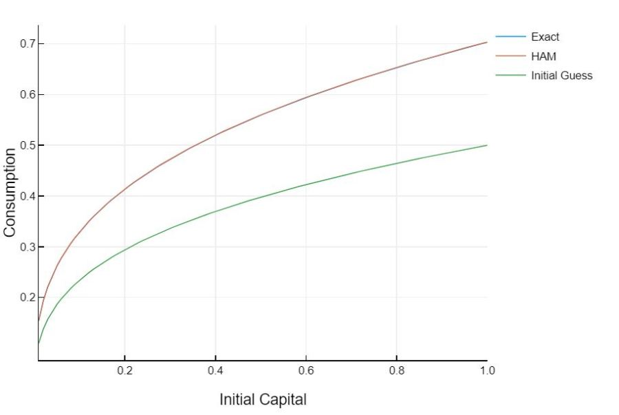
This is a special case where we know the exact solution to our problem. The solution to the baby growth model is $c(k) =(1-\beta \theta) k^{\theta}$ .

Consumption No Depre

Adding Depreciation

The baby growth model seemed a bit contrived. We already knew the functional form of the solution and so could make a good initial guess. If we add in depreciation however, we don’t have that same luxury. With depreciation, the optimal consumption rule will not be to consume a constant share of output. But that is okay. It will not materially impact our analysis or the good

Consumption with Depre

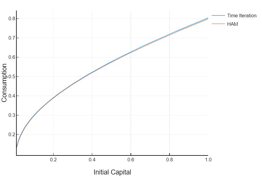
It appears that this approximation is worse than the no depreciation case, but it is actually the time iteration curve that is incorrect. My time iteration code is only set up to solve a model with a non-inelastic supply of labor. Instead of solving a model with utility

$u(c_t) = \ln c_t$

I’m actually solving a model with utility

$u(c_t, l_t) = \ln c_t + \gamma \ln l_t$

with $\gamma$ set near zero. So the approximation using the Homotopy Analysis Method is actually more precise. Notice that our initial guess for the solution, which was consuming a constant share of capital, does not have the same functional form as the solution. The Homotopy Analysis Method is deforming our initial guess until it gives an approximate analytic solution. This is in contrast to the full depreciation case, where the solution had the same functional form as our guess. This just goes to show that the Homotopy Analysis Method can give very accurate approximations even when we don’t know what form the solution will take.

One point that we haven’t discussed in depth is how to choose the convergence control parameter. Our approximations were very accurate but depended heavily on this constant. In the full-depreciation example the convergence control parameter was set to $-1.1$ but in the more general model we set it equal to $-0.375$ . This seems, and is, arbitrary. If we used higher order terms, so $x_3, x_4, x_5, ...$ etc. we would need to use a different convergence control parameter. If we had a different initial guess at $\alpha$ we would need to use a different parameter. If we used a different initial guess at the functional form we would need to use a different parameter. One of the strengths of HAM is that it is very flexible, but this makes it difficult to find generally applicable rules to use when choosing $H(k)$ , $h$ , and $\mathcal{L}$ , almost to the point that the method isn’t very useful. Here are the heuristic rules that I use when solving problems.

Ignore $\mathcal{L}$ unless derivatives appear in your nonlinear equation
Choose an initial guess that conforms with the boundary conditions of your problem (not heuristic, this is just necessary) and, if possible, lead to separable terms in the nonlinear equation
Choose $H(k)$ so that it eliminates the most terms in the nonlinear equation.
Choose $h$ so that the approximation evaluated at the steady-state returns the steady-state.

For $2$ , we want to choose $x_0(k)$ such that the nonlinear term is as simple as possible. In the growth model this resulted in consuming a constant fraction of output. The first nonlinear term, evaluated at $q = 0$ reduced to

$\beta \theta \left(k^{\theta} - \alpha k^{\theta} \right)^{\theta -1} = \beta \theta (1-\alpha)^{\theta-1}k^{\theta^2 - \theta}$

Notice how much simpler this term is than if we guessed $x_0(k) = k$ instead. Then we wouldn’t be able to work with just $k$ but would need to carry around $\left(k^{\theta} - k \right)^{\theta -1}$ in all of our calculations. Of course, with depreciation we will need to do this any ways, which brings us to point $3$ . Using a good auxiliary function can reduce the number of terms in $R_n$ that we need to calculate. By using

$H(k) = \left((1-\alpha)*\left(k^{\theta} + (1-\delta)k\right) \right)^{1-\theta}$

we just remove a term from $x_1$ entirely. This ultimately results in needing to calculate fewer derivatives for higher order approximations (remember that $x_2$ depends on the number of terms in $x_1$ , and so on). Finally, for point $4$ , we generally are able to easily calculate what the steady state is in our problems. We can therefore use this information to find the right convergence control parameter. If our approximation is at all good it should return the steady state consumption when evaluated at the steady state capital. We can choose $h$ to force this behavior at any level of approximation.

Basic Mechanics

SymEngine / SymPy

Baby Growth Model

Programming the Homotopy Analysis Method

Adding Depreciation

Share this:

Like this: